Note
Go to the end to download the full example code.
Stabilize Spacecraft
Objectives
Show the use of quaternions to represent orientation in a somewhat less than trivial example.
Show how to use additional equations for
optyin conjunction with variable bounds to force functions of the state to satisfy conditions along the trajectory.
Description
A spacecraft rotates in outer space where no gravity is present.
The spacecraft is modeled as a thin walled box of side lengths
\(l_1\), \(l_2\), and \(l_3\).
A linkage of mass \(m_l\) shaped as a T is rotably attached to the
the center of mass of the spacecraft. The length of the vertical part of
the T is denoted by \(b\) and the length of the horizontal part by
\(c\). Control torques \(t_x, t_y, t_z\) are applied to
it. A mass modeled as a homogenious box of mass \(m_m\) and
side lengths \(s_1, s_2, s_3\) can
move frictionlessly along the’horizontal part’ of the linkage. A
control force \(f_z\) and control torques \(t_{xp}, t_{yp}, t_{zp}\)
are applied to it.
The goal is to orient the spacecraft in such a way, that the body fixed frame of the spacecraft (A1) aligns with the inertial frame (N) in their z direction, that is no rotation around the x and y axes.
Notes
The idea is from https://arc.aiaa.org/doi/abs/10.2514/3.55956?journalCode=jgc which was written for another purpose. The linkage design is changed.
As there are no external forces or torques acting on the system, its angular momentum should be constant. The solution thus obtained did not keep it constant. When adding equations forcing it to be constant, it became constant. It seems unclear, whether such an enforcing helps or hurts the solution.
Solving the system as an ODE, with the controls replaced by simple functions only kept the angular momentum approximately constant when very small tolerances
atol, rtolwere used withsolve_ivp.No statements can be made about the kinetic energy of the system as confirmed by Carlos Roithmayr (private communication).
The objective function is to minimize the ‘total movement around the x and y axes of the spacecraft’, while it reaches the final position.
While 1.5.0 is the latest released version of opty, the developmental version must be used to run this code.
Using quaternions instead of Euler angles seems to reduce the time opty needs to get a solution quite a bit.
Final orientation of the spacecraft: With \(c_i = \cos(\dfrac{\theta_i}{2})\) and \(s_i = \sin(\dfrac{\theta_i}{2})\), where \(\theta_1, \theta_2, \theta_3\) are the Euler angles representing the rotation of the spacecraft in the XYZ convention, the relationship between the Euler angles and the quaternion is:
\(q_1 = s_1 c_2 c_3 + c_1 s_2 s_3\)
\(q_2 = c_1 s_2 c_3 - s_1 c_2 s_3\)
\(q_3 = c_1 c_2 s_3 + s_1 s_2 c_3\)
\(q_0^2 + q_1^2 + q_2^2 + q_3^2 = 1\), as q must be a unit quaternion.
Hence the requirement \(\theta_1(t_f) = \theta_2(t_f) = 0\) and \(\theta_3(t_f)\) arbitrary gives \(q_1(t_f) = q_2(t_f) = 0\). This is used in the instance constraints.
Increasing
fpsin the animation program will make the animation smooother at the expense of increased storage.
States
\(q_0, q_1, q_2, q_3\) : quaternion of the spacecraft’s body fixed frame (A1) relative to the inertial frame (N).
\(u_0, u_1, u_2, u_3\) : velocities
\(q_{00}, q_4, q_5, q_6\) : quaternion of the linkage’s body fixed frame (A2) relative to the spacecraft’s body fixed frame.
\(u_{00}, u_4, u_5, u_6\) : velocities.
\(q_{000}, q_7, q_8, a_9\) : quaternion of the mass’s body fixed frame (A3) relative to the linkage’s body fixed frame (A2).
\(u_{000}, u_7, u_8, u_9\) : velocities.
\(r, u_r\) : Position and velocity of the mass along the horizontal part (A2.z) of the linkage.
\(x_1, x_2, x_3\) : Position of the spacecraft’s center of mass in the inertial frame.
\(ux_1, ux_2, ux_3\) : Velocity of the spacecraft’s center of mass in the inertial frame.
Controls
\(t_x, t_y, t_z\) : Torques acting on the \(A2_x, A2_y, A2_z\) axes of the linkage.
\(f_z\) : Force acting on the mass along the \(A2_z\) axis of the linkage.
\(t_{xp}, t_{yp}, t_{zp}\) : Control torques acting on the \(A3_x, A3_y, A3_z\) axes of the mass.
Parameters
\(m\) : Mass of the spacecraft.
\(m_ l\) : Mass of the linkage.
\(m_m\) : Mass of the moving mass.
\(s_1, s_2, s_3\) : Side lengths of the moving mass.
\(b, c\) : Geometric parameters of the linkage.
\(l_1, l_2, l_3\) : side lengths of the spacecraft.
import sympy as sm
import sympy.physics.mechanics as me
import numpy as np
import matplotlib.pyplot as plt
import time
from scipy.interpolate import interp1d
from matplotlib.animation import FuncAnimation
from mpl_toolkits.mplot3d.art3d import Poly3DCollection
from opty.direct_collocation import Problem
Set up Kane’s Equations of Motion
Define the reference frames and points. Define the time symbols t. Set the speed of the reference point O to zero.
N, A1, A2, A3 = sm.symbols('N A1 A2 A3', cls=me.ReferenceFrame)
O, Dmc, P1, P2, P3 = sm.symbols('O Dmc P1 P2 P3', cls=me.Point)
t = me.dynamicsymbols._t
O.set_vel(N, 0)
Coordinates and speeds of Dmc.
x1, x2, x3, ux1, ux2, ux3 = me.dynamicsymbols('x1 x2 x3 ux1 ux2 ux3')
Rotation and angular velocity of the spacecraft, the linkge and the mass
q0, q1, q2, q3, q00, q4, q5, q6, q000, q7, q8, q9 = me.dynamicsymbols(
'q0 q1 q2 q3 q00 q4 q5 q6 q000 q7 q8 q9')
u0, u1, u2, u3, u00, u4, u5, u6, u000, u7, u8, u9 = me.dynamicsymbols(
'u0 u1 u2 u3 u00 u4 u5 u6 u000 u7 u8 u9')
Control inputs for opty.
tx, ty, tz, fz = me.dynamicsymbols('tx ty tz fz')
txp, typ, tzp = me.dynamicsymbols('txp typ tzp')
Position and speed of the moving mass.
r, ur = me.dynamicsymbols('r ur')
Parameters of the system.
m, mm, ml = sm.symbols('m mm ml')
b, c, l1, l2, l3 = sm.symbols('b c l1 l2 l3')
s1, s2, s3 = sm.symbols('s1 s2 s3')
Body fixed frame of the spacecraft.
A1.orient_quaternion(N, (q0, q1, q2, q3))
Body fixed frame of the linkage.
A2.orient_quaternion(A1, (q00, q4, q5, q6))
Body fixed frame of the mass
A3.orient_quaternion(A2, (q000, q7, q8, q9))
Mass center of the spacecraft.
Dmc.set_pos(O, x1 * N.x + x2 * N.y + x3 * N.z)
Dmc.set_vel(N, ux1 * N.x + ux2 * N.y + ux3 * N.z)
Point of the linkage where the upright part meets the horizontal part.
P2.set_pos(Dmc, b * A2.x)
P2.v2pt_theory(Dmc, N, A2)
print('angular velocity of A3 in A1:')
A3.ang_vel_in(A1)
angular velocity of A3 in A1:
(2*q00(t)*Derivative(q4(t), t) - 2*q4(t)*Derivative(q00(t), t) - 2*q5(t)*Derivative(q6(t), t) + 2*q6(t)*Derivative(q5(t), t))*A2.x + (2*q00(t)*Derivative(q5(t), t) + 2*q4(t)*Derivative(q6(t), t) - 2*q5(t)*Derivative(q00(t), t) - 2*q6(t)*Derivative(q4(t), t))*A2.y + (2*q00(t)*Derivative(q6(t), t) - 2*q4(t)*Derivative(q5(t), t) + 2*q5(t)*Derivative(q4(t), t) - 2*q6(t)*Derivative(q00(t), t))*A2.z + (2*q000(t)*Derivative(q7(t), t) - 2*q7(t)*Derivative(q000(t), t) - 2*q8(t)*Derivative(q9(t), t) + 2*q9(t)*Derivative(q8(t), t))*A3.x + (2*q000(t)*Derivative(q8(t), t) + 2*q7(t)*Derivative(q9(t), t) - 2*q8(t)*Derivative(q000(t), t) - 2*q9(t)*Derivative(q7(t), t))*A3.y + (2*q000(t)*Derivative(q9(t), t) - 2*q7(t)*Derivative(q8(t), t) + 2*q8(t)*Derivative(q7(t), t) - 2*q9(t)*Derivative(q000(t), t))*A3.z
Position of the mass moving on the horizontal part of the linkage.
P3.set_pos(P2, r * A2.z)
P3.set_vel(A2, ur * A2.z)
Inertia of a box with thin walls and side lengths \(l_1, l_2, l_3\) and mass \(m\) (from the internet).
iXX = m / (12*(l1*l2 + l2*l3 + l1*l3)) * (
l2**3 * (l1 + l3) + l3**3*(l1 + l2) + 3*l1*l2*l3*(l2 + l3))
iYY = m / (12*(l1*l2 + l2*l3 + l1*l3)) * (
l1**3 * (l2 + l3) + l3**3*(l1 + l2) + 3*l1*l2*l3*(l1 + l3))
iZZ = m / (12*(l1*l2 + l2*l3 + l1*l3)) * (
l1**3 * (l2 + l3) + l2**3*(l1 + l3) + 3*l1*l2*l3*(l1 + l2))
I_spacecraft = me.inertia(A1, iXX, iYY, iZZ)
spacecraft = me.RigidBody('spacecraft', Dmc, A1, m, (I_spacecraft, Dmc))
Inertia of homogenious brick with sides \(s_1, s_2, s_3\) and mass \(m_m\).
iXXp = mm / 12 * (s2**2 + s3**2)
iYYp = mm / 12 * (s1**2 + s3**2)
iZZp = mm / 12 * (s1**2 + s2**2)
I_masse = me.inertia(A3, iXXp, iYYp, iZZp)
masse = me.RigidBody('masse', P3, A3, mm, (I_masse, P3))
Inertia of the T shaped linkage with upright part of length \(b\) and crossbar of length \(c\) and mass \(m_l\).
m1 = ml * b / (b + c) # upright rod mass
m2 = ml * c / (b + c) # crossbar rod mass
iXXl = m2 * c**2 / 12
iYYl = m1 * b**2 / 3 + m2 * c**2 / 12
iZZl = m1 * b**2 / 3
I_linkage = me.inertia(A2, iXXl, iYYl, iZZl)
linkage = me.RigidBody('linkage', P2, A2, ml, (I_linkage, P2))
Assemble the list of bodies of the system.
bodies = [spacecraft, masse, linkage]
Forces and torques acting on the linkage and the mass, and the reaction forces acting on the spacecraft.
FL = [
(A2, tx*A2.x + ty*A2.y + tz*A2.z),
(A1, -tx*A2.x - ty*A2.y - tz*A2.z),
(A3, txp*A3.x + typ*A3.y + tzp*A3.z),
(A1, -txp*A3.x - typ*A3.y - tzp*A3.z),
(P3, fz*A2.z),
(Dmc, -fz*A2.z),
(A1, -P3.pos_from(Dmc).cross(fz*A2.z)),
]
Differential kinematic equations for the system.
kd = sm.Matrix([
q0.diff(t) - u0,
q1.diff(t) - u1,
q2.diff(t) - u2,
q3.diff(t) - u3,
q00.diff(t) - u00,
q4.diff(t) - u4,
q5.diff(t) - u5,
q6.diff(t) - u6,
q000.diff(t) - u000,
q7.diff(t) - u7,
q8.diff(t) - u8,
q9.diff(t) - u9,
r.diff(t) - ur,
x1.diff(t) - ux1,
x2.diff(t) - ux2,
x3.diff(t) - ux3,
])
Configuration constraints for the quaternions.
config_constr = sm.Matrix([
q0**2 + q1**2 + q2**2 + q3**2 - 1,
q00**2 + q4**2 + q5**2 + q6**2 - 1,
q000**2 + q7**2 + q8**2 + q9**2 - 1,
])
Speed constraints are obtained by differentiating the configuration constraints with respect to time. Needed for Kane’s method.
speed_constr = config_constr.diff(t)
Finish setting up Kane’s EOMs.
q_ind = [q1, q2, q3, q4, q5, q6, q7, q8, q9, r, x1, x2, x3]
q_dep = [q0, q00, q000]
u_ind = [u1, u2, u3, u4, u5, u6, u7, u8, u9, ur, ux1, ux2, ux3]
u_dep = [u0, u00, u000]
kane = me.KanesMethod(
N,
q_ind,
u_ind,
q_dependent=q_dep,
u_dependent=u_dep,
kd_eqs=kd,
configuration_constraints=config_constr,
velocity_constraints=speed_constr,
)
fr, frstar = kane.kanes_equations(bodies, FL)
eom = kd.col_join(fr + frstar)
Force the angular momentum to be constant, equal to its initial value.
H01, H02, H03 = sm.symbols('H01 H02 H03')
H_total = sum([b.angular_momentum(O, N) for b in bodies])
eom_H = sm.Matrix([H_total.dot(N.x) - H01,
H_total.dot(N.y) - H02,
H_total.dot(N.z) - H03])
eom = eom.col_join(eom_H)
Create a dictionary replacing the time derivatives of the generalized coordinates with their expressions from the kinematic differential equations.
A_kin, b_kin = sm.linear_eq_to_matrix(kd, [i.diff(t) for i in q_ind + q_dep])
loesung = A_kin.LUsolve(b_kin)
kin_dict = {i.diff(t): loesung[j] for j, i in enumerate(q_ind + q_dep)}
Force the x, y components of the angular velocity of A1 to be zero at \(t_f\).
A1_ang_x, A1_ang_y = me.dynamicsymbols('A1_ang_x A1_ang_y')
eom_ang = sm.Matrix([A1.ang_vel_in(N).dot(N.x) - A1_ang_x,
A1.ang_vel_in(N).dot(N.y) - A1_ang_y])
eom = eom.col_join(eom_ang)
Force the x, y components of the ang. accelerations to be zero at \(t_f\).
A1_ang_x_dot, A1_ang_y_dot = me.dynamicsymbols('A1_ang_x_dot A1_ang_y_dot')
A1_ang_vel = me.msubs(A1.ang_vel_in(N), kin_dict)
A1_ang_acc = A1_ang_vel.diff(t, N)
eom_ang_acc = sm.Matrix([A1_ang_acc.dot(N.x) - A1_ang_x_dot,
A1_ang_acc.dot(N.y) - A1_ang_y_dot])
eom = eom.col_join(eom_ang_acc)
Add the quaternion normalization constraints to the EOMs. This avoids their drift away from unit norm.
eom = eom.col_join(config_constr)
Define the position constraint for the auxiliary point. At the end N.z and A1.z should be aligned and point in the same direction.
P_hilfs = me.Point('P_hilfs')
dir_vec = me.dynamicsymbols('dir_vec')
P_hilfs.set_pos(Dmc, 1 * A1.z)
upright_eom = sm.Matrix([P_hilfs.pos_from(Dmc).dot(N.z) - dir_vec])
eom = eom.col_join(upright_eom)
Print information about the EOMs.
print(f"The eoms have {sm.count_ops(eom):,} operations"
f" {sm.count_ops(sm.cse(eom))} operations after cse")
print('Shape of the EOMs:', eom.shape)
The eoms have 455,368 operations 4006 operations after cse
Shape of the EOMs: (40, 1)
Compile some functions for later use.
qLL = q_ind + q_dep + u_ind + u_dep
pLL = [m, mm, ml, b, c, l1, l2, l3, s1, s2, s3]
Define the total angular momentum and its components.
H_total = sum([me.msubs(b.angular_momentum(O, N), kin_dict) for b in bodies])
moment = [H_total.dot(uv) for uv in N]
moment_lam = sm.lambdify(qLL + pLL, moment, cse=True)
Define the kinetic energy of the system, but keep in mind the notes above.
kin_energy = sum([me.msubs(body.kinetic_energy(N), kin_dict)
for body in bodies])
kin_lam = sm.lambdify(qLL + pLL, kin_energy, cse=True)
Initial rotations and speeds are given as angles and angle-speeds, convert then to quaternions and quaternion rates.
def euler123_quaternions(a, ad):
# a = [a1, a2, a3] Euler angles in body-fixed 1-2-3 sequence
# ad = [a1d, a2d, a3d] d/dt of Euler angles
# Returns q = [q0..q3] and qd = dq/dt.
# From the internet. Formulae likely in textbooks on quaternions.
a1, a2, a3 = a
a1d, a2d, a3d = ad
c1, s1 = np.cos(a1/2), np.sin(a1/2)
c2, s2 = np.cos(a2/2), np.sin(a2/2)
c3, s3 = np.cos(a3/2), np.sin(a3/2)
q0 = c1*c2*c3 - s1*s2*s3
q1 = s1*c2*c3 + c1*s2*s3
q2 = c1*s2*c3 - s1*c2*s3
q3 = c1*c2*s3 + s1*s2*c3
qd0 = -0.5*(q1*a1d + q2*a2d + q3*a3d)
qd1 = 0.5*(q0*a1d + (c1*c2*s3 - s1*s2*c3)*a2d + q2*a3d)
qd2 = 0.5*(-q3*a1d + (c1*c2*c3 + s1*s2*s3)*a2d - q1*a3d)
qd3 = 0.5*(q2*a1d + (s1*c2*c3 - c1*s2*s3)*a2d + q0*a3d)
return np.array([q0, q1, q2, q3]), np.array([qd0, qd1, qd2, qd3])
Set up for opty
state_symbols = q_ind + q_dep + u_ind + u_dep
num_nodes = 500
t0, tf = 0.0, 5.0
interval_value = (tf - t0) / (num_nodes - 1)
Set the parameters.
par_map = {}
par_map[m] = 1.0
par_map[mm] = 1.0
par_map[ml] = 0.1
par_map[b] = 0.5
par_map[c] = None
par_map[l1] = 2.0
par_map[l2] = 2.0
par_map[l3] = 2.0
par_map[s1] = 0.2
par_map[s2] = 0.4
par_map[s3] = 0.6
c_max = min(par_map[l1], par_map[l2], par_map[l3]) / 2.0
par_map[c] = c_max
Needed for lambdified functions later.
pL_vals = [par_map[i] for i in par_map.keys()]
Define the objective function:
The x and y components of the angular velocity of A1 w.r.t. the inertial frame N should be minimized. so the objective function is the sum of the squares of the x and y components of the angular velocity of A1 w.r.t. N. and the gradient function is the jacobian of the objective function with respect to the state symbols.
A1_ang = me.msubs(A1.ang_vel_in(N), kin_dict)
omega = me.msubs(sm.Matrix([A1_ang.dot(N.x)**2 +
A1_ang.dot(N.y)**2]), kin_dict)
omega_jac = omega.jacobian(state_symbols)
omega_lam = sm.lambdify(state_symbols + pLL, omega, cse=True)
omega_jac_lam = sm.lambdify(state_symbols + pLL, omega_jac, cse=True)
test = np.random.rand(len(state_symbols))
def obj(free):
summe = 0
params = np.empty(len(state_symbols))
for i in range(num_nodes):
params = np.array([free[i + j*num_nodes]
for j in range(len(state_symbols))])
summe += omega_lam(*params, *pL_vals).squeeze()
return summe * interval_value
def obj_grad(free):
grad = np.zeros_like(free)
for i in range(num_nodes):
params = np.array([free[i + j*num_nodes]
for j in range(len(state_symbols))])
omega_jac_vall = omega_jac_lam(*params, *pL_vals).squeeze()
for j in range(len(state_symbols)):
grad[i + j*num_nodes] = omega_jac_vall[j].squeeze()
return grad * interval_value
Limit of the control torques and force.
grenze = 25.0
This limits the velocity and acceleration for the last portion of the nodes of the angular velocity of A1 w.r.t. N and of its acceleration.
lim_low_vel = np.full(num_nodes, -np.inf)
lim_up_vel = np.full(num_nodes, np.inf)
lim_low_acc = np.full(num_nodes, -np.inf)
lim_up_acc = np.full(num_nodes, np.inf)
lim_vel = 5.0
lim_acc = 30.0
los = int(num_nodes * 0.9)
delta = num_nodes - los
lim_low_vel[los:] = np.array([(lim_vel / delta) * (i - los) - lim_vel
for i in range(los, num_nodes)])
lim_up_vel[los:] = np.array([(-lim_vel / delta) * (i - los) + lim_vel
for i in range(los, num_nodes)])
lim_low_acc[los:] = np.array([(lim_acc / delta) * (i - los) - lim_acc
for i in range(los, num_nodes)])
lim_up_acc[los:] = np.array([(-lim_acc / delta) * (i - los) + lim_acc
for i in range(los, num_nodes)])
N.z and A1.z should be aligned and point in the same direction.
lim_low_vec = np.full(num_nodes, -1.5)
lim_up_vec = np.full(num_nodes, 1.5)
los_vec = int(num_nodes * 0.99)
delta_vec = num_nodes - los_vec
lim_low_vec[los_vec:] = np.array([0.5 for i in range(los_vec, num_nodes)])
Define the bounds.
bounds = {
tx: (-grenze, grenze),
ty: (-grenze, grenze),
tz: (-grenze, grenze),
fz: (-grenze, grenze),
txp: (-grenze, grenze),
typ: (-grenze, grenze),
tzp: (-grenze, grenze),
r: (-0.25 * min(par_map[l1], par_map[l2], par_map[l3]),
0.25 * min(par_map[l1], par_map[l2], par_map[l3])),
A1_ang_x: (lim_low_vel, lim_up_vel),
A1_ang_y: (lim_low_vel, lim_up_vel),
A1_ang_x_dot: (lim_low_acc, lim_up_acc),
A1_ang_y_dot: (lim_low_acc, lim_up_acc),
dir_vec: (lim_low_vec, lim_up_vec),
}
Set the initial values for the states.
Given in degrees and then converted into quaternions / quaternion-speeds.
Initial rotations and speeds of A1 w.r.t. N
alpha = np.deg2rad(67.0)
beta = np.deg2rad(67.0)
gamma = np.deg2rad(67.0)
alpha_dot = 2.0
beta_dot = 2.0
gamma_dot = 2.0
q01q, q01d = euler123_quaternions([alpha, beta, gamma],
[alpha_dot, beta_dot, gamma_dot])
Initial rotations and speeds of A2 w.r.t. A1
alpha = 0.0
beta = 0.0
gamma = 0.0
alpha_dot = 0.0
beta_dot = 0.0
gamma_dot = 0.0
q001q, q001d = euler123_quaternions([alpha, beta, gamma],
[alpha_dot, beta_dot, gamma_dot])
Initial rotation and speeds of A3 w.r.t. A2
alpha = np.deg2rad(45.0)
beta = np.deg2rad(45.0)
gamma = np.deg2rad(45.0)
alpha_dot = 0.0
beta_dot = 0.0
gamma_dot = 0.0
q0000q, q0000d = euler123_quaternions([alpha, beta, gamma],
[alpha_dot, beta_dot, gamma_dot])
Set the initial values for the states.
q01, q11, q21, q31 = q01q
q001, q41, q51, q61 = q001q
q0001, q71, q81, q91 = q0000q
r1 = 0.0
x11 = 0.0
x21 = 0.0
x31 = 0.0
u01, u11, u21, u31 = q01d
u001, u41, u51, u61 = q001d
u0001, u71, u81, u91 = q0000d
ur1 = 0.0
ux11 = 0.0
ux21 = 0.0
ux31 = 0.0
instance_constraints = [
q0.func(t0) - q01,
q1.func(t0) - q11,
q2.func(t0) - q21,
q3.func(t0) - q31,
q00.func(t0) - q001,
q4.func(t0) - q41,
q5.func(t0) - q51,
q6.func(t0) - q61,
q000.func(t0) - q0001,
q7.func(t0) - q71,
q8.func(t0) - q81,
q9.func(t0) - q91,
r.func(t0) - r1,
x1.func(t0) - x11,
x2.func(t0) - x21,
x3.func(t0) - x31,
u0.func(t0) - u01,
u1.func(t0) - u11,
u2.func(t0) - u21,
u3.func(t0) - u31,
u00.func(t0) - u001,
u4.func(t0) - u41,
u5.func(t0) - u51,
u6.func(t0) - u61,
ur.func(t0) - ur1,
ux1.func(t0) - ux11,
ux2.func(t0) - ux21,
ux3.func(t0) - ux31,
q1.func(tf) - 0,
q2.func(tf) - 0,
]
Get values of the initial angular momentum components. The angular momentum must be equal to the initial values.
qL_vals = [q11, q21, q31, q41, q51, q61, q71, q81, q91, r1, x11, x21,
x31] + [q01, q001, q0001]
uL_vals = [u11, u21, u31, u41, u51, u61, u71, u81, u91, ur1, ux11, ux21,
ux31] + [u01, u001, u0001]
H_fix1, H_fix2, h_fix3 = moment_lam(*qL_vals, *uL_vals, *pL_vals)
par_map.update({H01: H_fix1, H02: H_fix2, H03: h_fix3})
Set up a Problem instance.
prob = Problem(
obj,
obj_grad,
eom,
state_symbols,
num_nodes,
interval_value,
known_parameter_map=par_map,
instance_constraints=instance_constraints,
bounds=bounds,
)
print('length of free vector: ', prob.num_free)
length of free vector: 22000
Solve the problem.
initial_guess = np.ones(prob.num_free)
prob.add_option('max_iter', 10000)
start_time = time.time()
solution, info = prob.solve(initial_guess)
print(info['status_msg'])
end_time = time.time()
minutes, seconds = divmod(end_time - start_time, 60)
print(f"Time needed to solve the problem: {int(minutes)} "
f"min {seconds:.2f} sec")
b'Algorithm stopped at a point that was converged, not to "desired" tolerances, but to "acceptable" tolerances (see the acceptable-... options).'
Time needed to solve the problem: 42 min 39.70 sec
Plot objective value.
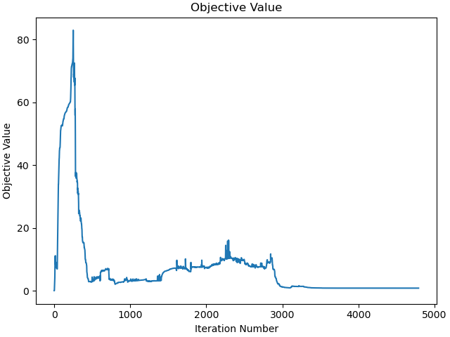
_ = prob.plot_objective_value()
Plot the jacobian of the problem.
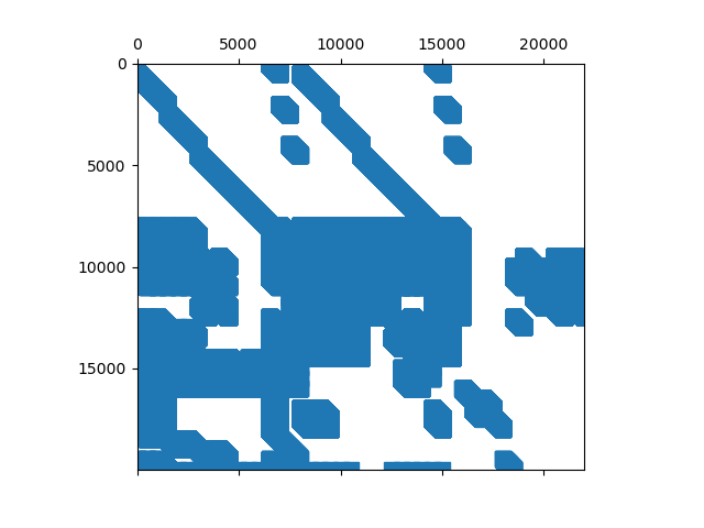
_ = prob.plot_jacobian_sparsity()
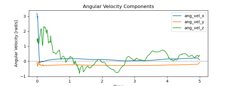
Plot the components of the angular velocity of the spacecraft.
ang_vel = me.msubs(A1.ang_vel_in(N), kin_dict)
ang_vel_components = [ang_vel.dot(uv) for uv in N]
ang_vel_lam = sm.lambdify(qLL + pLL, ang_vel_components, cse=True)
names = ['ang_vel_x', 'ang_vel_y', 'ang_vel_z']
resultat, *_ = prob.parse_free(solution)
times = prob.time_vector(solution)
fig, ax = plt.subplots(figsize=(8, 3))
for i, name in enumerate(names):
ax.plot(times, [ang_vel_lam(*resultat[:, j], *pL_vals)[i]
for j in range(resultat.shape[1])], label=names[i])
ax.set_xlabel('Time')
ax.set_ylabel('Angular Velocity [rad/s]')
ax.axhline(0.0, color='k', lw=0.5, ls='--')
ax.set_title('Angular Velocity Components')
_ = ax.legend()
Plot the state trajectories.
_ = prob.plot_trajectories(solution, show_bounds=True)

Plot the violations of the constraints.
_ = prob.plot_constraint_violations(solution, subplots=True)

How well is the angular momentum kept?
The first value is ignored, see opty issue #412.
resultat, *_, = prob.parse_free(solution)
H_total = sum([me.msubs(b.angular_momentum(O, N), kin_dict) for b in bodies])
moment = [H_total.dot(uv) for uv in N]
moment_lam = sm.lambdify(qLL + pLL, moment, cse=True)
pL_vals = [par_map[i] for i in pLL]
H_val = moment_lam(*resultat, *pL_vals)
delta1 = np.max(H_val[0][1:]) - np.min(H_val[0][1:])
delta2 = np.max(H_val[1][1:]) - np.min(H_val[1][1:])
delta3 = np.max(H_val[2][1:]) - np.min(H_val[2][1:])
delta_H = delta1 + delta2 + delta3
print("Max deviation in angular momentum components from being constant is: "
f"{delta_H:.3e}")
fig, ax = plt.subplots(2, 1, figsize=(8, 4), sharex=True, layout='constrained')
for i in range(3):
ax[0].plot(prob.time_vector(solution)[1:],
moment_lam(*resultat, *pL_vals)[i][1:],
label=f'H_{i+1}')
ax[0].set_title('Components of the angular momerntum')
ax[-1].set_xlabel('Time')
ax[0].legend()
ax[1].plot(prob.time_vector(solution), kin_lam(*resultat, *pL_vals))
_ = ax[1].set_title('Kinetic energy')
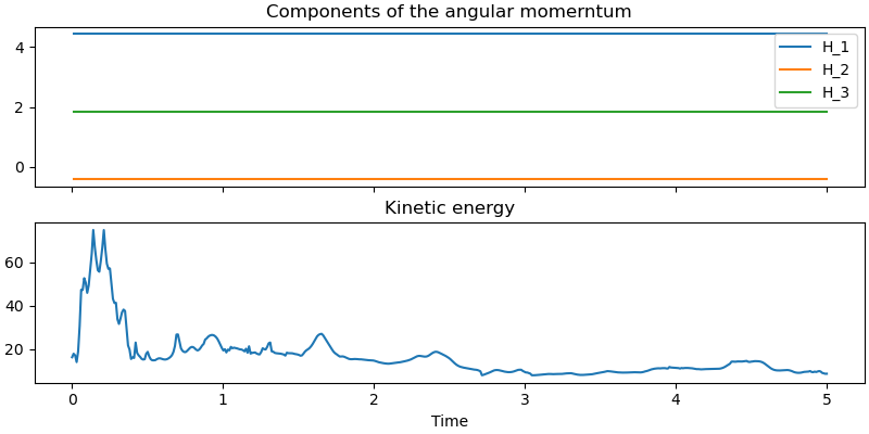
Max deviation in angular momentum components from being constant is: 9.957e-11
Revert back to Euler angles XYZ for the plot. Needed for the rotation of the spacecraft.
def quat_to_euler_xyz(q):
q = np.asarray(q, dtype=float)
q0, q1, q2, q3 = q
s2 = 2.0 * (q1*q3 + q0*q2)
# -1 <= s2 <= 1 needed because of arcsin.
s2 = np.clip(s2, -1.0, 1.0)
a2 = np.arcsin(s2)
a1 = np.arctan2(-2.0*(q2*q3 - q0*q1), 1.0 - 2.0*(q1**2 + q2**2))
a3 = np.arctan2(-2.0*(q1*q2 - q0*q3), 1.0 - 2.0*(q2**2 + q3**2))
return [a1, a2, a3]
Compute the quaternion representing the rotation of frame A3 relative to frame A1. This is the Hamilton product of the quaternions: \({}^{A1}q^{A3} = {}^{A1}q^{A2} \otimes {}^{A2}q^{A3}\)
def quat_A3_in_A1(A2_in_A1, A3_in_A2):
# Get the rotation quaternion of A3 relative to A1
q00, q4, q5, q6 = A2_in_A1
q000, q7, q8, q9 = A3_in_A2
r0 = q00*q000 - q4*q7 - q5*q8 - q6*q9
r1 = q00*q7 + q4*q000 + q5*q9 - q6*q8
r2 = q00*q8 - q4*q9 + q5*q000 + q6*q7
r3 = q00*q9 + q4*q8 - q5*q7 + q6*q000
return [r0, r1, r2, r3]
Animation
The motion of the center of mass is suppressed to better see the rotations. The rotating box was written by AI. I just adapted it to my needs.
v_ang = me.msubs(A1.ang_vel_in(N), kin_dict)
v_ang = [v_ang.dot(uv) for uv in N]
v_ang_lam = sm.lambdify(qLL + pLL, v_ang, cse=True)
# Start the animation program.
fps = 10
resultat, *_ = prob.parse_free(solution)
# Interpolation of the solution
t_arr = prob.time_vector(solution)
y_arr = resultat
state_sol = interp1d(
t_arr,
y_arr,
kind="cubic",
axis=1
)
# End points of the horizontal part of the T linkage.
P_T1, P_T2 = sm.symbols('P_T1 P_T2', cls=me.Point)
P_T1.set_pos(P2, par_map[c] / 2 * A2.z)
P_T2.set_pos(P2, -par_map[c] / 2 * A2.z)
coordinates = Dmc.pos_from(O).to_matrix(N)
for point in (P2, P3, P_T1, P_T2):
coordinates = coordinates.row_join(point.pos_from(O).to_matrix(N))
coordinates_lam = sm.lambdify(qLL + pLL, coordinates, cse=True)
# Spacecraft dimensions in the animation
l11 = par_map[l1]
l21 = par_map[l2]
l31 = par_map[l3]
# mass dimensions in the animation
s11 = par_map[s1]
s21 = par_map[s2]
s31 = par_map[s3]
alpha_space = 0.25
alpha_mass = 0.25
def euler_angles_A1(t):
winkel = quat_to_euler_xyz([state_sol(t)[13], state_sol(t)[0],
state_sol(t)[1], state_sol(t)[2]])
q11, q21, q31 = winkel
return q11, q21, q31
def euler_angles_A3(t):
A2_in_A1 = [state_sol(t)[13], state_sol(t)[0], state_sol(t)[1],
state_sol(t)[2]]
A3_in_A2 = [state_sol(t)[14], state_sol(t)[3], state_sol(t)[4],
state_sol(t)[5]]
rot = quat_A3_in_A1(A2_in_A1, A3_in_A2)
winkel = quat_to_euler_xyz(rot)
q13, q23, q33 = winkel
return q13, q23, q33
# Kinematics
def R1(q):
c, s = np.cos(q), np.sin(q)
return np.array([[1, 0, 0], [0, c, -s], [0, s, c]])
def R2(q):
c, s = np.cos(q), np.sin(q)
return np.array([[c, 0, s], [0, 1, 0], [-s, 0, c]])
def R3(q):
c, s = np.cos(q), np.sin(q)
return np.array([[c, -s, 0], [s, c, 0], [0, 0, 1]])
def rotation_matrix_NA(q1, q2, q3):
"""Rotation matrix from A to N (body-fixed 1-2-3 sequence)."""
return R1(q1) @ R2(q2) @ R3(q3)
# Corner points in A1 relative to Dmc (rows = points)
h1 = np.array([l11, l21, l31]) / 2.0
corners_A1 = np.array([[sx * h1[0], sy * h1[1], sz * h1[2]]
for sx in (-1, 1) for sy in (-1, 1) for sz in (-1, 1)])
# Corner points in A3 relative to P3
h3 = np.array([s11, s21, s31]) / 2.0
corners_A3 = np.array([[sx * h3[0], sy * h3[1], sz * h3[2]]
for sx in (-1, 1) for sy in (-1, 1) for sz in (-1, 1)])
# Faces as index lists into the corners
# (pairs of opposite faces share a colour)
faces_idx = [
[0, 1, 3, 2], [4, 5, 7, 6], # -e1 / +e1
[0, 1, 5, 4], [2, 3, 7, 6], # -e2 / +e2
[0, 2, 6, 4], [1, 3, 7, 5], # -e3 / +e3
]
face_colors1 = ["tab:red"] * 2 + ["tab:green"] * 2 + ["tab:blue"] * 2
face_colors2 = ["tab:grey"] * 2 + ["tab:grey"] * 2 + ["tab:grey"] * 2
# Edges (for a clean wireframe)
edges_idx = [(0, 1), (2, 3), (4, 5), (6, 7),
(0, 2), (1, 3), (4, 6), (5, 7),
(0, 4), (1, 5), (2, 6), (3, 7)]
def pose_A1(t):
"""Return corners in N, centre M in N, and rotation matrix R_NA."""
R1 = rotation_matrix_NA(*euler_angles_A1(t))
M1 = (0.0, 0.0, 0.0)
corners_N1 = M1 + corners_A1 @ R1.T
return corners_N1, M1, R1
def pose_A3(t):
"""Return corners in N, centre P3 in N, and rotation matrix R_NA3."""
R3 = rotation_matrix_NA(*euler_angles_A3(t))
P3 = (coordinates_lam(*state_sol(t), *pL_vals)[:, 2] -
coordinates_lam(*state_sol(t), *pL_vals)[:, 0])
corners_N3 = P3 + corners_A3 @ R3.T
return corners_N3, P3, R3
times = np.concatenate((np.arange(0.0, tf, 1.0 / fps), [tf]))
fig = plt.figure(figsize=(9, 8))
ax = fig.add_subplot(111, projection="3d")
ax.set_xlabel("$N_1$ [m]")
ax.set_ylabel("$N_2$ [m]")
ax.set_zlabel("$N_3$ [m]")
r_max = 0.5 * np.linalg.norm([l11, l21, l31])
lo = -r_max
hi = +r_max
ctr = 0.5 * (lo + hi)
half = 0.5 * (hi - lo)
ax.set_xlim(-half, half)
ax.set_ylim(-half, half)
ax.set_zlim(-half, half)
ax.set_box_aspect((1, 1, 1))
# Translucent faces
c01, _, _ = pose_A1(0.0)
poly1 = Poly3DCollection([c01[f] for f in faces_idx],
facecolors=face_colors1, edgecolors="k",
linewidths=1.0, alpha=alpha_space)
ax.add_collection3d(poly1)
c03, _, _ = pose_A3(0.0)
poly3 = Poly3DCollection([c03[f] for f in faces_idx],
facecolors=face_colors2, edgecolors="k",
linewidths=1.0, alpha=alpha_mass)
ax.add_collection3d(poly3)
# Body-fixed axes of A (drawn from M)
axis_len = 1.0 * max(l11, l21, l31)
axis_colors = ["tab:red", "tab:green", "tab:blue"]
axis_lines = [ax.plot([], [], [], color=col, lw=0.5)[0] for col in axis_colors]
axis_labels = [ax.text(0, 0, 0, f"$A1_{i+1}$", color=axis_colors[i])
for i in range(3)]
# Inertial frame N at origin
for i, (col, lab) in enumerate(zip("rgb", ["N1", "N2", "N3"])):
d = np.zeros(3)
d[i] = half * 0.4
ax.plot([0, d[0]], [0, d[1]], [0, d[2]], color=col, lw=1, ls="--",
alpha=0.6)
# Centre of mass
com_dot, = ax.plot([], [], [], "ko", ms=5)
trail, = ax.plot([], [], [], "k-", lw=1, alpha=0.5)
title = ax.set_title("")
# Create P2, P3
pt2, = ax.plot([], [], [], 'o', color='blue', markersize=5)
pt3, = ax.plot([], [], [], 'o', color='black', markersize=5)
# Create the lines connecting Dmc to P2 and P2 to P3
line2, = ax.plot([], [], [], '-', color='red', lw=2.5)
line3, = ax.plot([], [], [], '-', color='red', lw=2.5)
# create the arrow showing angular velocity
arrow_head = np.array(
[v_ang_lam(*state_sol(0), *pL_vals)[0] -
coordinates_lam(*state_sol(0), *pL_vals)[0, 0],
v_ang_lam(*state_sol(0), *pL_vals)[1] -
coordinates_lam(*state_sol(0), *pL_vals)[1, 0],
v_ang_lam(*state_sol(0), *pL_vals)[2] -
coordinates_lam(*state_sol(0), *pL_vals)[2, 0]])
arrow = ax.quiver(*[0.0, 0.0, 0.0], *arrow_head,
arrow_length_ratio=0.15,
color='green', linewidth=2)
def update(k):
global arrow
t = times[k]
corners_N1, M1, R1 = pose_A1(t)
poly1.set_verts([corners_N1[f] for f in faces_idx])
corners_N3, *_ = pose_A3(t)
poly3.set_verts([corners_N3[f] for f in faces_idx])
for i, line in enumerate(axis_lines):
tip = M1 + axis_len * R1[:, i]
line.set_data_3d([M1[0], tip[0]], [M1[1], tip[1]], [M1[2], tip[2]])
axis_labels[i].set_position_3d(tip)
q1, q2, q3 = euler_angles_A1(t)
title.set_text(f"Running time = {t:4.2f} sec \n "
" Angles of rotation of the spacecraft = "
f"({np.degrees(q1):.0f}°,"
f" {np.degrees(q2):.0f}°, {np.degrees(q3):.0f}°) \n"
"The small box ist the mass moved around to stabilize "
"the spacecraft. \n The green arrow gives the"
f" angular velocity of the spacecraft. \n"
"The red lines are the T shaped linkage.")
# Update the positions of P2, P3, and the connecting lines
coords = coordinates_lam(*state_sol(t), *pL_vals)
p2x = coords[0, 1] - coords[0, 0]
p2y = coords[1, 1] - coords[1, 0]
p2z = coords[2, 1] - coords[2, 0]
pt2.set_data_3d([p2x], [p2y], [p2z])
p3x = coords[0, 2] - coords[0, 0]
p3y = coords[1, 2] - coords[1, 0]
p3z = coords[2, 2] - coords[2, 0]
pt3.set_data_3d([p3x], [p3y], [p3z])
pT1x = coords[0, 3] - coords[0, 0]
pT1y = coords[1, 3] - coords[1, 0]
pT1z = coords[2, 3] - coords[2, 0]
pT2x = coords[0, 4] - coords[0, 0]
pT2y = coords[1, 4] - coords[1, 0]
pT2z = coords[2, 4] - coords[2, 0]
line2.set_data_3d([p2x, 0.0], [p2y, 0.0], [p2z, 0.0])
line3.set_data_3d([pT1x, pT2x], [pT1y, pT2y], [pT1z, pT2z])
# As quiver cannot be updated easily in 3D remove the old arrow and
# create a new one
arrow.remove()
arrow_head = (np.array([v_ang_lam(*state_sol(t), *pL_vals)[0],
v_ang_lam(*state_sol(t), *pL_vals)[1],
v_ang_lam(*state_sol(t), *pL_vals)[2]]))
arrow = ax.quiver(*[0.0, 0.0, 0.0], *arrow_head,
arrow_length_ratio=0.15,
color='green', linewidth=2)
return (poly1, poly3, com_dot, trail, *axis_lines, pt2, pt3,
line2, line3, arrow)
anim = FuncAnimation(fig, update, frames=len(times),
interval=1500 / fps, blit=False)
plt.show()