Note
Go to the end to download the full example code.
Parameter Identification with Non-Contiguous Measurements.
Objective
Show how to use opty to estimate parameters of a mechanical system from noisy measurements.
Show a way to handle explicit time in the equations of motion (very small point)
Description
For parameter estimation it is common to collect measurements of a system’s trajectories for distinct experiments. For example, if you are identifying the parameters of a mass-spring-damper system, you will excite the system with different initial conditions multiple times. The data cannot simply be stacked and the identification run because the measurement data would be discontinuous between trials.
A work around in opty is to create a set of differential equations with unique state variables for each measurement trial that all share the same constant parameters. You can then identify the parameters from all measurement trials simultaneously by passing the uncoupled differential equations to opty.
For example:
number_of_measurements measurements of the location of a simple system consisting of a mass connected to a fixed point by a spring and a damper, with a force = \(F_1 \sin(\omega \cdot t)\) acting on the mass. The movement is in a horizontal direction. \(c, F_1, k, \omega\) are to be identified.
Notes
This is just a slightly more elaborate version of an example from opty: https://opty.readthedocs.io/stable/examples/intermediate/plot_non_contiguous_parameter_identification.html#sphx-glr-examples-intermediate-plot-non-contiguous-parameter-identification-py
State Variables
\(x_i\): position of the mass of the i - th measurement trial [m]
\(u_i\): speed of the mass of the i - th measurement trial [m/s]
Parameters
\(m\): mass [kg]
\(c\): damping coefficient [Ns/m]
\(k\): spring constant [N/m]
\(l_0\): natural length of the spring [m]
\(F_1\): amplitude of the force [N]
\(\omega\): frequency of the force [rad/s]
Set up the equations of motion and integrate them to get the measurements.
import sympy as sm
import numpy as np
import sympy.physics.mechanics as me
import matplotlib.pyplot as plt
from scipy.integrate import solve_ivp
from opty import Problem

number_of_measurements = 15
t0, tf = 0, 10
num_nodes = 400
times = np.linspace(t0, tf, num_nodes)
t_span = (t0, tf)
np.random.seed(1234)

x = me.dynamicsymbols(f'x:{number_of_measurements}')
u = me.dynamicsymbols(f'u:{number_of_measurements}')
fx = me.dynamicsymbols('f_x')
m, c, k, l0 = sm.symbols('m, c, k, l0')
F1, omega = sm.symbols('F1, omega')
t = me.dynamicsymbols._t
T = me.dynamicsymbols('T')

eom1 = sm.Matrix([x[i].diff(t) - u[i] for i in range(number_of_measurements)])
eom2 = sm.Matrix([m*u[i].diff(t) + c*u[i] + k*(x[i] - l0) -
                  F1*sm.sin(omega*T)
                  for i in range(number_of_measurements)])
eom = eom1.col_join(eom2)
Print the equations of motion.
sm.pprint(eom)
⎡ d ⎤
⎢ -u₀(t) + ──(x₀(t)) ⎥
⎢ dt ⎥
⎢ ⎥
⎢ d ⎥
⎢ -u₁(t) + ──(x₁(t)) ⎥
⎢ dt ⎥
⎢ ⎥
⎢ d ⎥
⎢ -u₂(t) + ──(x₂(t)) ⎥
⎢ dt ⎥
⎢ ⎥
⎢ d ⎥
⎢ -u₃(t) + ──(x₃(t)) ⎥
⎢ dt ⎥
⎢ ⎥
⎢ d ⎥
⎢ -u₄(t) + ──(x₄(t)) ⎥
⎢ dt ⎥
⎢ ⎥
⎢ d ⎥
⎢ -u₅(t) + ──(x₅(t)) ⎥
⎢ dt ⎥
⎢ ⎥
⎢ d ⎥
⎢ -u₆(t) + ──(x₆(t)) ⎥
⎢ dt ⎥
⎢ ⎥
⎢ d ⎥
⎢ -u₇(t) + ──(x₇(t)) ⎥
⎢ dt ⎥
⎢ ⎥
⎢ d ⎥
⎢ -u₈(t) + ──(x₈(t)) ⎥
⎢ dt ⎥
⎢ ⎥
⎢ d ⎥
⎢ -u₉(t) + ──(x₉(t)) ⎥
⎢ dt ⎥
⎢ ⎥
⎢ d ⎥
⎢ -u₁₀(t) + ──(x₁₀(t)) ⎥
⎢ dt ⎥
⎢ ⎥
⎢ d ⎥
⎢ -u₁₁(t) + ──(x₁₁(t)) ⎥
⎢ dt ⎥
⎢ ⎥
⎢ d ⎥
⎢ -u₁₂(t) + ──(x₁₂(t)) ⎥
⎢ dt ⎥
⎢ ⎥
⎢ d ⎥
⎢ -u₁₃(t) + ──(x₁₃(t)) ⎥
⎢ dt ⎥
⎢ ⎥
⎢ d ⎥
⎢ -u₁₄(t) + ──(x₁₄(t)) ⎥
⎢ dt ⎥
⎢ ⎥
⎢ d ⎥
⎢ -F₁⋅sin(ω⋅T(t)) + c⋅u₀(t) + k⋅(-l₀ + x₀(t)) + m⋅──(u₀(t)) ⎥
⎢ dt ⎥
⎢ ⎥
⎢ d ⎥
⎢ -F₁⋅sin(ω⋅T(t)) + c⋅u₁(t) + k⋅(-l₀ + x₁(t)) + m⋅──(u₁(t)) ⎥
⎢ dt ⎥
⎢ ⎥
⎢ d ⎥
⎢ -F₁⋅sin(ω⋅T(t)) + c⋅u₂(t) + k⋅(-l₀ + x₂(t)) + m⋅──(u₂(t)) ⎥
⎢ dt ⎥
⎢ ⎥
⎢ d ⎥
⎢ -F₁⋅sin(ω⋅T(t)) + c⋅u₃(t) + k⋅(-l₀ + x₃(t)) + m⋅──(u₃(t)) ⎥
⎢ dt ⎥
⎢ ⎥
⎢ d ⎥
⎢ -F₁⋅sin(ω⋅T(t)) + c⋅u₄(t) + k⋅(-l₀ + x₄(t)) + m⋅──(u₄(t)) ⎥
⎢ dt ⎥
⎢ ⎥
⎢ d ⎥
⎢ -F₁⋅sin(ω⋅T(t)) + c⋅u₅(t) + k⋅(-l₀ + x₅(t)) + m⋅──(u₅(t)) ⎥
⎢ dt ⎥
⎢ ⎥
⎢ d ⎥
⎢ -F₁⋅sin(ω⋅T(t)) + c⋅u₆(t) + k⋅(-l₀ + x₆(t)) + m⋅──(u₆(t)) ⎥
⎢ dt ⎥
⎢ ⎥
⎢ d ⎥
⎢ -F₁⋅sin(ω⋅T(t)) + c⋅u₇(t) + k⋅(-l₀ + x₇(t)) + m⋅──(u₇(t)) ⎥
⎢ dt ⎥
⎢ ⎥
⎢ d ⎥
⎢ -F₁⋅sin(ω⋅T(t)) + c⋅u₈(t) + k⋅(-l₀ + x₈(t)) + m⋅──(u₈(t)) ⎥
⎢ dt ⎥
⎢ ⎥
⎢ d ⎥
⎢ -F₁⋅sin(ω⋅T(t)) + c⋅u₉(t) + k⋅(-l₀ + x₉(t)) + m⋅──(u₉(t)) ⎥
⎢ dt ⎥
⎢ ⎥
⎢ d ⎥
⎢-F₁⋅sin(ω⋅T(t)) + c⋅u₁₀(t) + k⋅(-l₀ + x₁₀(t)) + m⋅──(u₁₀(t))⎥
⎢ dt ⎥
⎢ ⎥
⎢ d ⎥
⎢-F₁⋅sin(ω⋅T(t)) + c⋅u₁₁(t) + k⋅(-l₀ + x₁₁(t)) + m⋅──(u₁₁(t))⎥
⎢ dt ⎥
⎢ ⎥
⎢ d ⎥
⎢-F₁⋅sin(ω⋅T(t)) + c⋅u₁₂(t) + k⋅(-l₀ + x₁₂(t)) + m⋅──(u₁₂(t))⎥
⎢ dt ⎥
⎢ ⎥
⎢ d ⎥
⎢-F₁⋅sin(ω⋅T(t)) + c⋅u₁₃(t) + k⋅(-l₀ + x₁₃(t)) + m⋅──(u₁₃(t))⎥
⎢ dt ⎥
⎢ ⎥
⎢ d ⎥
⎢-F₁⋅sin(ω⋅T(t)) + c⋅u₁₄(t) + k⋅(-l₀ + x₁₄(t)) + m⋅──(u₁₄(t))⎥
⎣ dt ⎦
Equations of motion for the solve_ivp integration.
rhs1 = np.array([u[i] for i in range(number_of_measurements)])
rhs2 = np.array([1/m * (-c*u[i] - k*(x[i] - l0) + F1*sm.sin(omega*t))
                 for i in range(number_of_measurements)])
rhs = np.concatenate((rhs1, rhs2))

qL = x + u
pL = [m, c, k, l0, F1, omega, t]

rhs_lam = sm.lambdify(qL + pL, rhs)


def gradient(t, x, args):
    args[-1] = t
    return rhs_lam(*x, *args).reshape(2 * number_of_measurements)


# Different initial conditions for the different measurements.
x0 = np.array([2 + (i / 4) * (-1)**i for i in range(number_of_measurements)] +
              [0 for _ in range(number_of_measurements)])
pL_vals = [1.0, 0.25, 2.0, 1.0, 6.0, 3.0, t0]

resultat1 = solve_ivp(gradient, t_span, x0, t_eval=times, args=(pL_vals,))
resultat = resultat1.y.T
Create the noisy measurements: simply add noise to the results of the integration.It is assumed, that only the locations are measured, not the speeds.
measurements = []

for i in range(number_of_measurements):
    measurements.append(resultat[:, i] + np.random.randn(resultat.shape[0]) *
                        1.0 / (i / 20 + 1) + np.random.randn(1) * 1.0 /
                        (i / 20 + 1))
Set up the Estimation Problem.
The idea is Gauss’ method of least squares: https://en.wikipedia.org/wiki/Least_squares
If some measurement is considered more reliable, its weight w may be increased.
objective = \(\int_{t_0}^{t_f} \left[ \sum_{i=1}^{ \textrm{number_of_measurements}} (w_i \cdot (x_i - x_i^m)^2 \right] dt\)
# This is added to get the explicit time for opty.
eom = eom.col_join(sm.Matrix([T.diff(t) - 1]))
state_symbols = x + u + [T]

interval_value = (tf - t0) / (num_nodes - 1)

par_map = {m: pL_vals[0],
           l0: pL_vals[3],
           }

# Weight vector. Here measurements with higher order number are considered
# more reliable, so their weight is set to be larger.
w = [1 + i for i in range(number_of_measurements)]


def obj(free):
    return interval_value * np.sum([w[i] * np.sum(
        (free[i*num_nodes:(i+1)*num_nodes] - measurements[i])**2)
        for i in range(number_of_measurements)])


def obj_grad(free):
    grad = np.zeros_like(free)
    for i in range(number_of_measurements):
        grad[i*num_nodes: (i+1)*num_nodes] = 2*w[i]*interval_value*(
            free[i*num_nodes:(i+1)*num_nodes] - measurements[i]
        )
    return grad


bounds = {
    c: (0, 1),
    k: (1, 3),
    F1: (5, 10),
    omega: (2, 7),
}

instance_constraints = (
                        T.func(t0) - 0.0,
                        )

problem = Problem(
    obj,
    obj_grad,
    eom,
    state_symbols,
    num_nodes,
    interval_value,
    known_parameter_map=par_map,
    instance_constraints=instance_constraints,
    bounds=bounds,
    time_symbol=me.dynamicsymbols._t,
)
This gives the unknown parameters, and their sequence in the solution vector.
print('unknown parameters are:', problem.collocator.unknown_parameters)
unknown parameters are: (F1, c, k, omega)
Initial guess.
list1 = [list(measurements[i]) for i in range(number_of_measurements)]
list1 = list(np.array(list1).flat)
initial_guess = np.array(
    list1
    + list(np.zeros(number_of_measurements*num_nodes))
    + list(np.linspace(t0, tf, num_nodes))
    + [0, 0, 0, 0]
)
Solve the Optimization Problem.
solution, info = problem.solve(initial_guess)
print(info['status_msg'])
_ = problem.plot_objective_value()
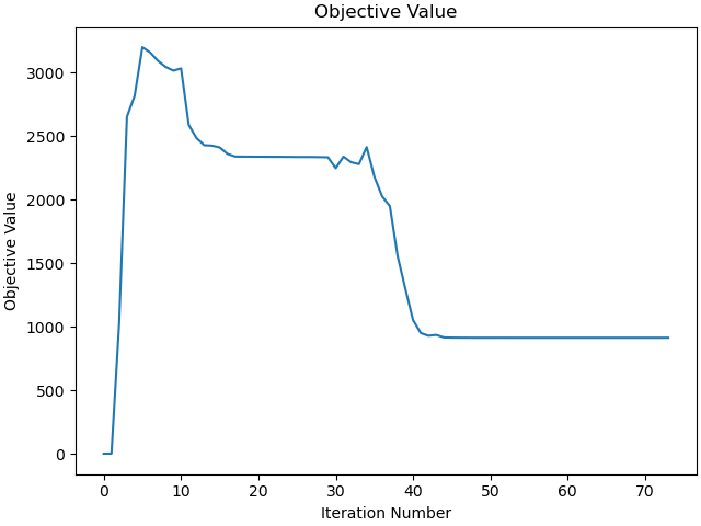
b'Algorithm terminated successfully at a locally optimal point, satisfying the convergence tolerances (can be specified by options).'
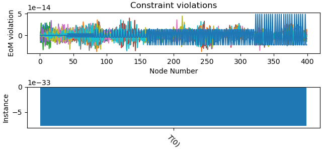
_ = problem.plot_constraint_violations(solution)
Results obtained
print('As the true values are known in this example, an error can be given')
print(f'Estimate of dampening constant is {solution[-3]:.2f} error is '
      f'{(solution[-3] - pL_vals[1])/pL_vals[1] * 100:.2f} %')
print(f'Estimate of spring constant is    {solution[-2]:.2f} error is '
      f'{(solution[-2] - pL_vals[2])/pL_vals[2] * 100:.2f} %')
print(f'Estimate of force is              {solution[-4]:.2f} error is '
      f'{(solution[-4] - pL_vals[4])/pL_vals[4] * 100:.2f} %')
print(f'Estimate of the frequency is      {solution[-1]:.2f} error is '
      f'{(solution[-1] - pL_vals[5])/pL_vals[5] * 100:.2f} %')
As the true values are known in this example, an error can be given
Estimate of dampening constant is 0.21 error is -14.30 %
Estimate of spring constant is    1.98 error is -1.01 %
Estimate of force is              5.93 error is -1.25 %
Estimate of the frequency is      2.99 error is -0.48 %
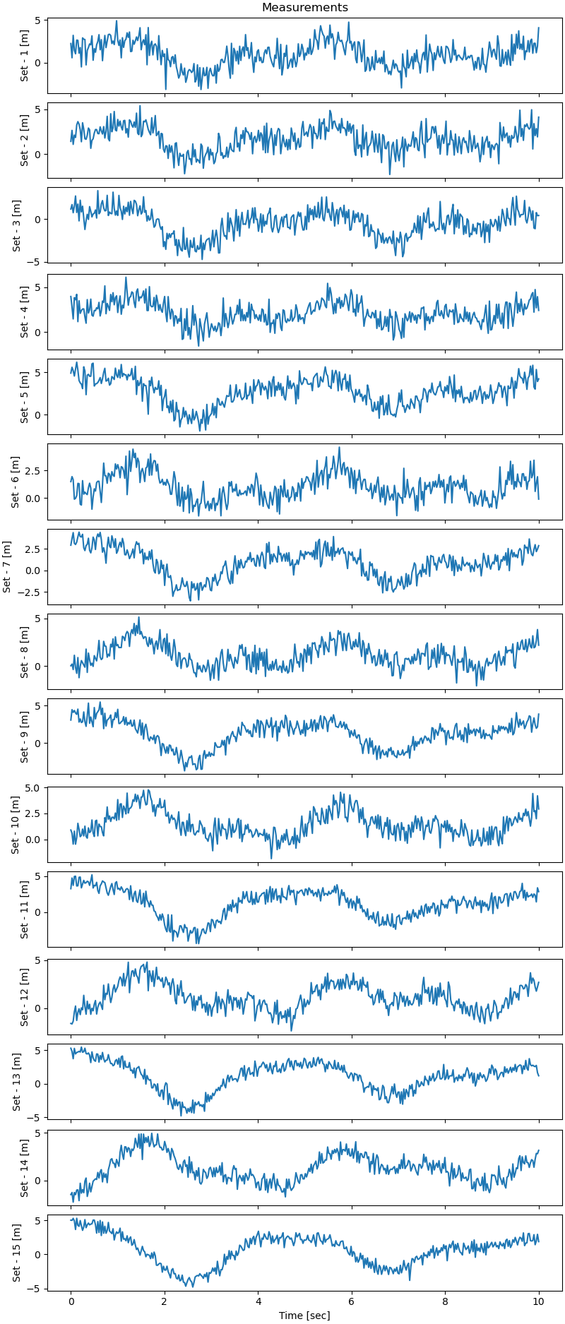
Plot the measurements.
fig, ax = plt.subplots(number_of_measurements, 1,
                       figsize=(8, 1.25 * number_of_measurements),
                       sharex=True, layout='constrained')
for i in range(number_of_measurements):
    ax[i].plot(times, measurements[i])
    ax[i].set_ylabel(f'Set - {i+1} [m]')
ax[0].set_title('Measurements')
_ = ax[-1].set_xlabel('Time [sec]')

plt.show()
Total running time of the script: (0 minutes 22.450 seconds)