Note
Go to the end to download the full example code.
Sailboat Around Buoy
Objective:
opty presently does not allow that intermediate instance constraints are
reached at times optimized by opty. This shows a way around this.
Description:
A boat is modeled as a rectangular plate with length \(a_B\) and width \(b_B\). It has a mass \(m_B\) and is modeled as a rigid body. At its stern there is a rudder of length \(l_R\). At its center there is a sail of length \(l_S\). Both may be rotated. As everything is two dimensional, I model them as thin rods. The wind blows in the positive Y direction, with constant speed \(v_W\). The water is at rest. Gravity, in the negative Z direction, is unimportant here, hence disregarded. (The dimensions of \(c_S, c_B\) come about because my ‘areas’ are one - dimensional).
Explanation how the task described above is achieved:
The boat should come close to two points, but opty should specify
the time when it should be there.
As presently with opty intermediate points must be specified as
\(t_{\textrm{intermediate}} = \textrm{integer}
\cdot \textrm{interval}_{\textrm{value}}\),
with \(0 < \textrm{integer} < num_{\textrm{nodes}}\) fixed, so this is
done:
Specify the points as \((x_{b_1}, y_{b_1}), (x_{b_2}, y_{b_2})\) and an allowable ‘radius’ called epsilon around these points.
Define a differentiable function \(hump(x, a, b, g_r)\) such that it is one for \(a \leq x \leq b\) and zero otherwise. \(g_r > 0\) is a parameter that determines how ‘sharp’ the transition is, the larger the sharper.
In order to know at the end of the run whether the boat came close to the point during its course, integrate the hump function over time. This is the variables \(\textrm{punkt}_1\) with \(\textrm{punkt}_1 = \int_{t0}^{tf} hump(...) \, dt > 0\) if the boat came close to the point, = 0 otherwise.
The exact values of \(\textrm{punkt}_1, \textrm{punkt}_2\) are not important as long as they are positive ‘enough’ , so define additional state variables \(\textrm{dist}_1, \textrm{dist}_2\) and specified variables \(h_1, h_2\).
by setting \(\textrm{dist}_1 = \textrm{punkt}_1 \cdot h_1\) and bounding \(h_1 \in (1, \textrm{value})\), and setting \(\textrm{dist}_1(t_f) = 1\), it can be ensured that \(\textrm{punkt}_1 > \dfrac{1}{\textrm{value}}\). Similar for \(\textrm{punkt}_2\).
Notes:
The idea is taken from: https://opty.readthedocs.io/stable/examples/advanced/plot_car_around_pylons.html#sphx-glr-examples-advanced-plot-car-around-pylons-py Only here the equations of motion are more complex, so convergence is more difficult.
The equations of motion were set up to the best of my ability, but I did not check them against a possibly more accurate model maybe available in some paper.
Constants
\(m_B\): mass of the boat [kg]
\(m_R\): mass of the rudder [kg]
\(m_S\): mass of the sail [kg]
\(l_R\): length of the rudder [m]
\(l_S\): length of the sail [m]
\(a_B\): length of the boat [m]
\(b_B\): width of the boat [m]
\(d_M\): distance of the mast from the center of the boat [m]
\(c_S\): drag coefficient at the sail [kg*sec/m^3]
\(c_B\): drag coefficient at boat and the rudder [kg*sec/m^3]
\(v_W\): speed of the wind [m/s]
\(\epsilon\): radius of a circle around the buoy [m]
\(x_{b_1}, y_{b_1}\): position of the buoy 1 [m]
\(x_{b_2}, y_{b_2}\): position of the buoy 2 [m]
States
\(x\): X - position of the center of the boat [m]
\(y\): Y - position of the center of the boat [m]
\(q_B\): angle of the boat [rad]
\(q_{S}\): angle of the sail [rad]
\(q_{R}\): angle of the rudder [rad]
\(u_x\): speed of the boat in X direction [m/s]
\(u_y\): speed of the boat in Y direction [m/s]
\(u_B\): angular speed of the boat [rad/s]
\(u_{R}\): angular speed of the rudder [rad/s]
\(u_{S}\): angular speed of the sail [rad/s]
\(\textrm{punkt}_1\): needed to get the boat close to the buoy 1
\(\textrm{punkt}_2\): needed to get the boat close to the buoy 2
\(\textrm{punkt}_{dt_1}\): needed to get the boat close to the buoy 1
\(\textrm{punkt}_{dt_2}\): needed to get the boat close to the buoy 2
\(\textrm{dist}_1\): needed to get the boat close to the buoy 1
\(\textrm{dist}_2\): needed to get the boat close to the buoy 2
Specifieds
\(t_{R}\): torque applied to the rudder [Nm]
\(t_{S}\): torque applied to the sail [Nm]
\(\textrm{dist}_{h_1}\): needed to get the boat close to buoy 1
\(\textrm{dist}_{h_2}\): needed to get the boat close to buoy 2
import numpy as np
import sympy as sm
import sympy.physics.mechanics as me
import matplotlib.pyplot as plt
import time
from opty.utils import parse_free
from scipy.interpolate import CubicSpline
from opty.direct_collocation import Problem
from matplotlib.animation import FuncAnimation
from matplotlib.patches import Rectangle, Circle
Set up the Equations of Motion
Set up the geometry of the system.
\(N\): inertial frame of reference
\(O\): origin of the inertial frame of reference
\(A_B\): body fixed frame of the boat
\(A_{R}\): body fixed frame of the rudder
\(A_{S}\): body fixed frame of the sail
\(A^{o}_B\): mass center of the boat
\(A^{o}_{R}\): mass center of the rudder
\(A^{o}_{RB}\): point where the rudder is attached to the boat
\(A^{o}_{S}\): mass center of the sail
N, AB, AR, AS = sm.symbols('N, AB, AR, AS', cls=me.ReferenceFrame)
O, AoB, AoR, AoS, AoRB = sm.symbols('O, AoB, AoR, AoS, AoRB', cls=me.Point)
qB, qR, qS, x, y = me.dynamicsymbols('qB, qR, qS, x, y')
uB, uR, uS, ux, uy = me.dynamicsymbols('uB, uR, uS, ux, uy')
tR, tS = me.dynamicsymbols('tR, tS')
mB, mR, mS, aB, bB, lR, lS = sm.symbols('mB, mR, mS, aB, bB, lR, lS',
real=True)
cB, cS, vW, dM = sm.symbols('cB, cS, vW, dM', real=True)
t = me.dynamicsymbols._t
O.set_vel(N, 0)
AB.orient_axis(N, qB, N.z)
AB.set_ang_vel(N, uB*N.z)
AR.orient_axis(AB, qR, N.z)
AR.set_ang_vel(AB, uR*N.z)
AS.orient_axis(AB, qS, N.z)
AS.set_ang_vel(AB, uS*N.z)
AoB.set_pos(O, x*N.x + y*N.y)
AoB.set_vel(N, ux*N.x + uy*N.y)
AoS.set_pos(AoB, dM*AB.y)
AoS.v2pt_theory(AoB, N, AB)
AoS.set_vel(N, AoB.vel(N))
AoRB.set_pos(AoB, -aB/2*AB.y)
AoRB.v2pt_theory(AoB, N, AB)
AoR.set_pos(AoRB, -lR/2*AR.y)
AoR.v2pt_theory(AoRB, N, AR)
test = 0
Set up the Drag Forces
The drag force acting on a body moving in a fluid is given by \(F_D = -\dfrac{1}{2} \rho C_D A | \bar v|^2 \hat v\), where \(C_D\) is the drag coefficient, \(\bar v\) is the velocity, \(\rho\) is the density of the fluid, \(\hat v\) is the unit vector of the velocity of the body and \(A\) is the cross section area of the body facing the flow. This may be found here:
https://courses.lumenlearning.com/suny-physics/chapter/5-2-drag-forces/
I will lump \(\dfrac{1}{2} \rho C_D\) into a single constant \(c\). (In the code below, I will use \(c_R\) for the boat and the rudder and \(c_S\) for the sails.) In order to avoid numerical issues functions not differentiable everywhere I will use the following:
\(F_{D_x} = -c A (\hat{A}.x \cdot \bar v)^2 \cdot \operatorname{sgn}(\hat{A}.x \cdot \bar v) \hat{A}.x\)
\(F_{D_y} = -c A (\hat{A}.y \cdot \bar v)^2 \cdot \operatorname{sgn}(\hat{A}.y \cdot \bar v) \hat{A}.y\)
As an (infinitely often) differentiable approximation of the sign function, I will use the fairly standard approximation:
\(\operatorname{sgn}(x) \approx \tanh( \alpha \cdot x )\) with \(\alpha \gg 1\)
Drag force acting on the boat.
helpx = AoB.vel(N).dot(AB.x)
helpy = AoB.vel(N).dot(AB.y)
FDBx = -cB*aB*(helpx**2)*sm.tanh(20*helpx)*AB.x
FDBy = -cB*bB*(helpy**2)*sm.tanh(20*helpy)*AB.y
forces = [(AoB, FDBx + FDBy)]
Drag force acting on the sail.
The effective wind speed on the sail is: \(v_W \hat{N}.y - (\bar{v}_B \cdot \hat{N}.y) \hat{N}.y\).
The width of the sail is negligible otherwise similar to the boat.
v_eff = vW*N.y - AoB.vel(N).dot(N.y)*N.y
FDSB = cS*lS*(v_eff.dot(AS.y)**2)*sm.tanh(20*v_eff.dot(AS.y))*AS.y
forces.append((AoS, FDSB))
Drag force acting on the rudder.
This is similar to the drag force on the boat, except the width of the rudder is negligible.
helpx = AoR.vel(N).dot(AR.x)
FDRx = -cB*lR*(helpx**2)*sm.tanh(20*helpx)*AR.x
forces.append((AoR, FDRx))
If \(u \neq 0\), the boat rotates and a drag torque acts on it. Let’s look at the situation from the center of the boat to its bow. At a distance \(r\) from the center, The speed of a point a r is \(u_B \cdot r\). The area is \(dr\), hence the force is \(-c_B (u_B r)^2 dr\). The lever at this point is \(r\), hence the torque is \(-c_B (u_B r)^2 r dr\). Hence total torque is:
\(-c_B u_B^2 \int_{0}^{a_B/2} r^3 \, dr\) = \(\frac{1}{4} c_B u_B^2 \dfrac{a_B^4}{16}\)
The same is from the center to the stern, hence the total torque due to \(a_B\) is \(\frac{1}{32} c_B u_B^2 a_B^4\).
Same again across the bow / stern, with \(b_B\) instead of \(a_B\), hence the total torque due to \(b_B\) is \(\frac{1}{32} c_B u_B^2 b_B^4\).
tB = -cB*uB**2*(aB**4 + bB**4)/32 * sm.tanh(20*uB) * N.z
forces.append((AB, tB))
Set control torques.
forces.append((AR, tR*N.z))
forces.append((AS, tS*N.z))
Set up the rigid bodies.
iZZ1 = 1/12 * mR * lR**2
iZZ2 = 1/12 * mS * lS**2
I1 = me.inertia(AR, 0, 0, iZZ1)
I2 = me.inertia(AS, 0, 0, iZZ2)
rudder = me.RigidBody('rudder', AoR, AR, mR, (I1, AoR))
sail = me.RigidBody('sail', AoS, AS, mS, (I2, AoRB))
iZZ = 1/12 * mB*(aB**2 + bB**2)
I3 = me.inertia(AB, 0, 0, iZZ)
boat = me.RigidBody('boat', AoS, AS, mS, (I3, AoS))
bodies = [boat, rudder, sail]
Set up Kane’s equations of motion.
q_ind = [qB, qR, qS, x, y]
u_ind = [uB, uR, uS, ux, uy]
kd = sm.Matrix([i - j.diff(t) for j, i in zip(q_ind, u_ind)])
KM = me.KanesMethod(N,
q_ind=q_ind,
u_ind=u_ind,
kd_eqs=kd,
)
fr, frstar = KM.kanes_equations(bodies, forces)
eom = kd.col_join(fr + frstar)
Set up the additional equations of motion to get close to the buoys.
def hump(x, a, b, gr):
# approx zero for x in [a, b]
# approx one otherwise
# the higher gr the closer the approximation
return 1.0 - (1/(1 + sm.exp(gr*(x - a))) + 1/(1 + sm.exp(-gr*(x - b))))
def step_l_diff(a, b, gr):
# approx zero for a < b, approx one otherwise
return 1/(1 + sm.exp(-gr*(a - b)))
def step_r_diff(a, b, gr):
# approx zero for a > b, approx one otherwise
return 1/(1 + sm.exp(gr*(a - b)))
xb1, yb1 = sm.symbols('xb1 yb1')
xb2, yb2 = sm.symbols('xb2 yb2')
punkt1, punktdt1 = me.dynamicsymbols('punkt1 punktdt1')
punkt2, punktdt2 = me.dynamicsymbols('punkt2 punktdt2')
dist1, disth1 = me.dynamicsymbols('dist1 disth1')
dist2, disth2 = me.dynamicsymbols('dist2 disth2')
epsilon, cutoff = sm.symbols('epsilon cutoff')
trog1 = (hump(x, xb1-epsilon, xb1+epsilon, cutoff) *
hump(y, yb1-epsilon, yb1+epsilon, cutoff))
trog2 = (hump(x, xb2-epsilon, xb2+epsilon, cutoff) *
hump(y, yb2-epsilon, yb2+epsilon, cutoff))
eom_add = sm.Matrix([
-punkt1.diff(t) + punktdt1,
-punktdt1 + trog1,
-dist1 + punkt1 * disth1,
-punkt2.diff(t) + punktdt2,
-punktdt2 + trog2,
-dist2 + punkt2 * disth2,
])
eom = eom.col_join(eom_add)
print(f' eom has shape {eom.shape} and has {sm.count_ops(eom)} operations')
eom has shape (16, 1) and has 1199 operations
Set up the Optimization Problem and Solve It
state_symbols = [qB, qR, qS, x, y, uB, uR, uS, ux, uy,
punkt1, punktdt1, dist1,
punkt2, punktdt2, dist2]
specified_symbols = [tR, tS, disth1, disth2]
constant_symbols = [mB, mR, mS, aB, bB, lR, lS, cB, cS, vW, dM,
xb1, yb1, xb2, yb2, epsilon]
num_nodes = 301
h = sm.symbols('h')
Specify the known symbols.
par_map = {}
par_map[mB] = 500.0
par_map[mR] = 10.0
par_map[mS] = 10.0
par_map[aB] = 10.0
par_map[bB] = 2.0
par_map[lR] = 2.0
par_map[lS] = 20.0
par_map[cB] = 1.0
par_map[cS] = 0.005
par_map[vW] = 25.0
par_map[dM] = -2.0
par_map[xb1] = 50.0
par_map[yb1] = 50.0
par_map[xb2] = 30.0
par_map[yb2] = 20.0
par_map[epsilon] = 2.0
par_map[cutoff] = 1.0
Set up the objective function and its gradient. The duration of the motion
is to be minimized, that is h, the last entry in free.
def obj(free):
return free[-1]
def obj_grad(free):
grad = np.zeros_like(free)
grad[-1] = 1.0
return grad
duration = (num_nodes - 1)*h
t0, tf = 0.0, duration
interval_value = h
Set up the instance constraints and the bounds.
instance_constraints = (
qB.func(t0) - 0.0,
qR.func(t0) - 0.0,
qS.func(t0) - 0.0,
x.func(t0) - 0.0,
y.func(t0) - 0.0,
uB.func(t0) - 0.0,
uR.func(t0) - 0.0,
uS.func(t0) - 0.0,
ux.func(t0) - 0.0,
uy.func(t0) - 0.0,
punkt1.func(t0) - 0.0,
punkt2.func(t0) - 0.0,
x.func(tf) - 0.0,
y.func(tf) - 0.0,
dist1.func(tf) - 1.0,
dist2.func(tf) - 1.0,
)
limit_torque = 100.0
bounds = {
tR: (-limit_torque, limit_torque),
tS: (-limit_torque, limit_torque),
qR: (-np.pi/2, np.pi/2),
qS: (0.0, np.pi/2),
h: (0.0, 3.0),
disth1: (1.0, 50.0),
disth2: (1.0, 50.0),
}
Only for the correct length of the initial guess.
prob = Problem(
obj,
obj_grad,
eom,
state_symbols,
num_nodes,
interval_value,
time_symbol=t,
known_parameter_map=par_map,
instance_constraints=instance_constraints,
backend='numpy',
bounds=bounds,
)
Pick a reasonable initial guess.
np.random.seed(10)
initial_guess = np.random.rand(prob.num_free)
sx1 = np.linspace(0, par_map[xb1], int(0.25*num_nodes))
sx2 = np.linspace(par_map[xb1], par_map[xb2],
int(0.5*num_nodes) - int(0.25*num_nodes))
sx3 = np.linspace(par_map[xb2], 0, num_nodes - int(0.5*num_nodes))
sy1 = np.linspace(0, par_map[yb1], int(0.25*num_nodes))
sy2 = np.linspace(par_map[yb1], par_map[yb2],
int(0.5*num_nodes) - int(0.25*num_nodes))
sy3 = np.linspace(par_map[yb2], 0, num_nodes - int(0.5*num_nodes))
initial_guess[3*num_nodes:4*num_nodes] = \
np.concatenate((sx1, sx2, sx3)).squeeze()
initial_guess[4*num_nodes:5*num_nodes] = \
np.concatenate((sy1, sy2, sy3)).squeeze()
initial_guess[-1] = 0.1
initial_guess = np.ones(prob.num_free)
Solve the Problem
Iterate from the second buoy close to the first buoy to the actual position further away.
zeit = time.time()
for i in range(15):
par_map[xb2] = 48.0 - i*2
par_map[yb2] = 48.0 - i*3.0
prob = Problem(
obj,
obj_grad,
eom,
state_symbols,
num_nodes,
interval_value,
time_symbol=t,
known_parameter_map=par_map,
instance_constraints=instance_constraints,
bounds=bounds,
tmp_dir='tmp_sailboat_around_buoy'
)
solution, info = prob.solve(initial_guess)
if info['status'] == 0:
print(f'after {i} iterations: {info["status_msg"]}')
print(f'Optimal h value is: {solution[-1]:.3f} sec')
initial_guess = solution
after 0 iterations: b'Algorithm terminated successfully at a locally optimal point, satisfying the convergence tolerances (can be specified by options).'
Optimal h value is: 0.340 sec
after 1 iterations: b'Algorithm terminated successfully at a locally optimal point, satisfying the convergence tolerances (can be specified by options).'
Optimal h value is: 0.340 sec
after 2 iterations: b'Algorithm terminated successfully at a locally optimal point, satisfying the convergence tolerances (can be specified by options).'
Optimal h value is: 0.340 sec
after 3 iterations: b'Algorithm terminated successfully at a locally optimal point, satisfying the convergence tolerances (can be specified by options).'
Optimal h value is: 0.340 sec
after 4 iterations: b'Algorithm terminated successfully at a locally optimal point, satisfying the convergence tolerances (can be specified by options).'
Optimal h value is: 0.340 sec
after 5 iterations: b'Algorithm terminated successfully at a locally optimal point, satisfying the convergence tolerances (can be specified by options).'
Optimal h value is: 0.340 sec
after 6 iterations: b'Algorithm terminated successfully at a locally optimal point, satisfying the convergence tolerances (can be specified by options).'
Optimal h value is: 0.340 sec
after 7 iterations: b'Algorithm terminated successfully at a locally optimal point, satisfying the convergence tolerances (can be specified by options).'
Optimal h value is: 0.340 sec
after 8 iterations: b'Algorithm terminated successfully at a locally optimal point, satisfying the convergence tolerances (can be specified by options).'
Optimal h value is: 0.340 sec
after 9 iterations: b'Algorithm terminated successfully at a locally optimal point, satisfying the convergence tolerances (can be specified by options).'
Optimal h value is: 0.340 sec
after 10 iterations: b'Algorithm terminated successfully at a locally optimal point, satisfying the convergence tolerances (can be specified by options).'
Optimal h value is: 0.340 sec
after 11 iterations: b'Algorithm terminated successfully at a locally optimal point, satisfying the convergence tolerances (can be specified by options).'
Optimal h value is: 0.340 sec
after 12 iterations: b'Algorithm terminated successfully at a locally optimal point, satisfying the convergence tolerances (can be specified by options).'
Optimal h value is: 0.340 sec
after 13 iterations: b'Algorithm terminated successfully at a locally optimal point, satisfying the convergence tolerances (can be specified by options).'
Optimal h value is: 0.340 sec
after 14 iterations: b'Algorithm terminated successfully at a locally optimal point, satisfying the convergence tolerances (can be specified by options).'
Optimal h value is: 0.340 sec
Now iterate on the sharpness of the hump function.
for i in range(5):
par_map[cutoff] = 1 + i*2.0
prob = Problem(
obj,
obj_grad,
eom,
state_symbols,
num_nodes,
interval_value,
time_symbol=t,
known_parameter_map=par_map,
instance_constraints=instance_constraints,
bounds=bounds,
tmp_dir='tmp_sailboat_around_buoy'
)
solution, info = prob.solve(initial_guess)
if info['status'] == 0:
print(f'after {i} iterations: {info["status_msg"]}')
print(f'Optimal h value is: {solution[-1]:.3f} sec')
initial_guess = solution
_ = prob.plot_objective_value()
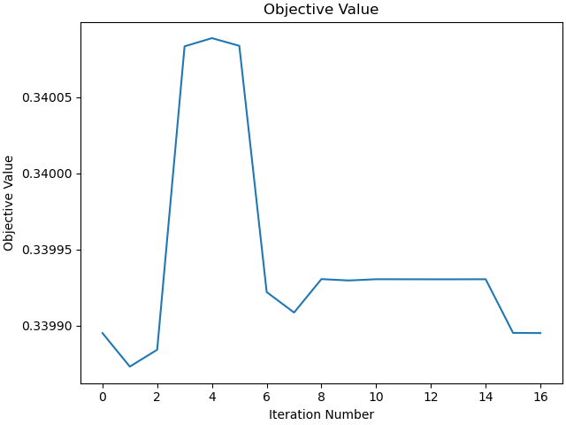
after 0 iterations: b'Algorithm terminated successfully at a locally optimal point, satisfying the convergence tolerances (can be specified by options).'
Optimal h value is: 0.340 sec
after 1 iterations: b'Algorithm terminated successfully at a locally optimal point, satisfying the convergence tolerances (can be specified by options).'
Optimal h value is: 0.340 sec
after 2 iterations: b'Algorithm terminated successfully at a locally optimal point, satisfying the convergence tolerances (can be specified by options).'
Optimal h value is: 0.340 sec
after 3 iterations: b'Algorithm terminated successfully at a locally optimal point, satisfying the convergence tolerances (can be specified by options).'
Optimal h value is: 0.340 sec
after 4 iterations: b'Algorithm terminated successfully at a locally optimal point, satisfying the convergence tolerances (can be specified by options).'
Optimal h value is: 0.340 sec
Time taken to find a solution.
print(f'Time taken to find a solution: {time.time() - zeit:.2f} sec')
Time taken to find a solution: 128.01 sec
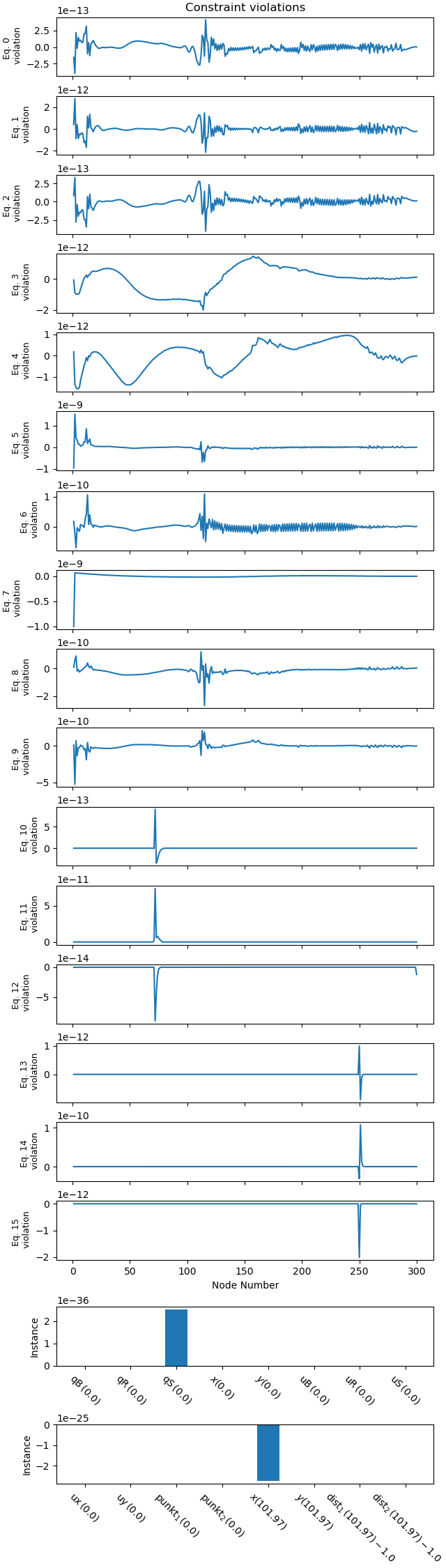
Plot errors in the solution.
_ = prob.plot_constraint_violations(solution, subplots=True)
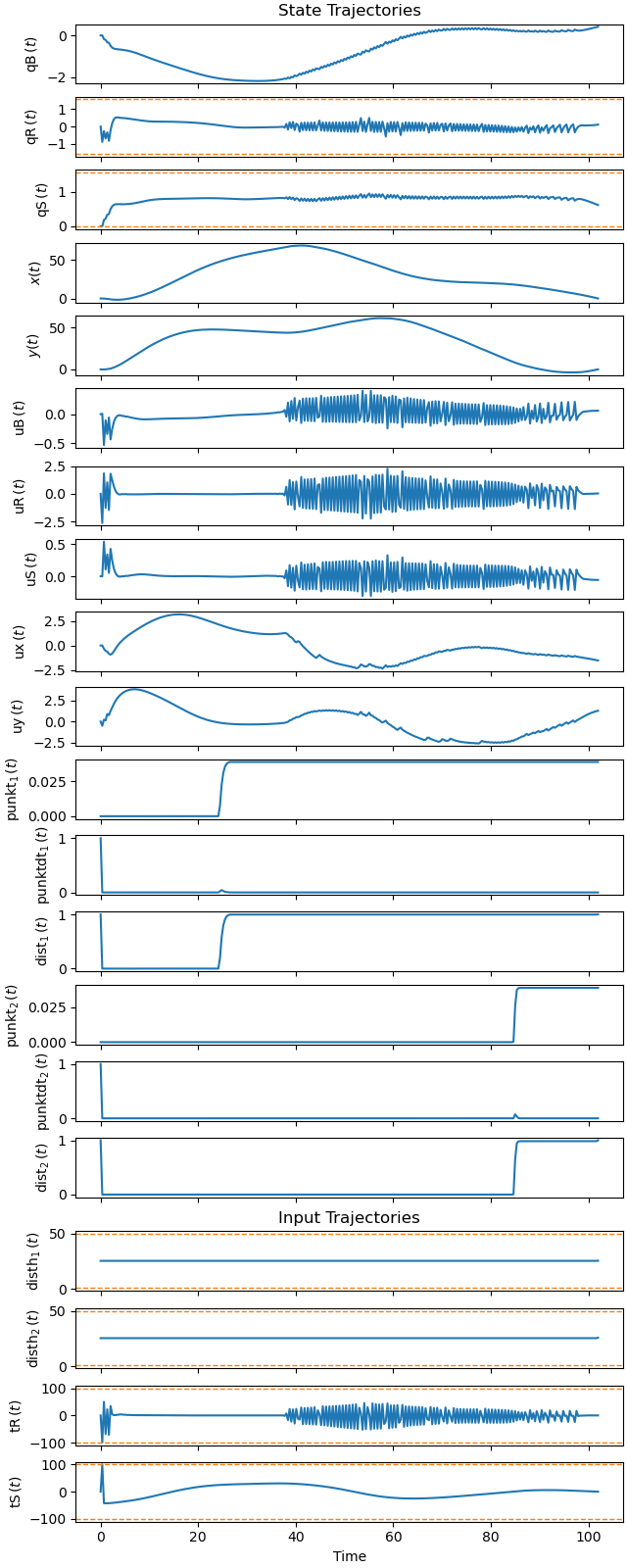
Plot the trajectories of the solution.
_ = prob.plot_trajectories(solution, show_bounds=True)
Animate the Solution
fps = 1.5
def add_point_to_data(line, x, y):
# to trace the path of the point.
old_x, old_y = line.get_data()
line.set_data(np.append(old_x, x), np.append(old_y, y))
state_vals, input_vals, _ = parse_free(solution, len(state_symbols),
len(specified_symbols), num_nodes)
t_arr = np.linspace(t0, num_nodes*solution[-1], num_nodes)
state_sol = CubicSpline(t_arr, state_vals.T)
input_sol = CubicSpline(t_arr, input_vals.T)
xmin = np.min(state_vals[3, :]) - par_map[aB]
xmax = np.max(state_vals[3, :]) + par_map[aB]
ymin = np.min(state_vals[4, :]) - par_map[aB]
ymax = np.max(state_vals[4, :]) + par_map[aB]
# additional points to plot the sail and the rudder
pRB, pSL, pSR = sm.symbols('pRB, pSL, pSR', cls=me.Point)
pRB.set_pos(AoRB, -lR*AR.y)
pSL.set_pos(AoS, -lS/2*AS.x)
pSR.set_pos(AoS, lS/2*AS.x)
coordinates = AoB.pos_from(O).to_matrix(N)
for point in (AoRB, pRB, pSL, pSR, AoS):
coordinates = coordinates.row_join(point.pos_from(O).to_matrix(N))
pL, pL_vals = zip(*par_map.items())
coords_lam = sm.lambdify(list(state_symbols) + [tR, tS, disth1, disth2] +
list(pL), coordinates, cse=True)
def init_plot():
fig, ax = plt.subplots(figsize=(6, 6), layout='constrained')
ax.set_xlim(xmin, xmax)
ax.set_ylim(ymin, ymax)
ax.set_aspect('equal')
ax.set_xlabel('x', fontsize=15)
ax.set_ylabel('y', fontsize=15)
circle1 = Circle((par_map[xb1], par_map[yb1]), par_map[epsilon] + 0.2,
edgecolor='blue', facecolor='none', linewidth=1)
ax.add_patch(circle1)
circle2 = Circle((par_map[xb2], par_map[yb2]), par_map[epsilon] + 0.2,
edgecolor='red', facecolor='none', linewidth=1)
ax.add_patch(circle2)
# draw the wind
X = np.linspace(xmin, xmax, 18)
Y = np.linspace(ymin, ymax, 18)
X1, Y1 = np.meshgrid(X, Y)
U = np.zeros_like(X1)
V = np.ones_like(Y1)
airflow = ax.quiver(X1, Y1, U, V, color='blue', scale=100.0, width=0.002,
alpha=0.5)
# draw the sail and the rudder
line1, = ax.plot([], [], lw=1, marker='o', markersize=0, color='green',
alpha=1.0)
line2, = ax.plot([], [], lw=1, marker='o', markersize=0, color='black')
line3 = ax.scatter([], [], color='black', s=10)
line4, = ax.plot([], [], lw=0.5, color='black')
boat = Rectangle((0 - par_map[bB]/2, 0 - par_map[aB]/2), par_map[bB],
par_map[aB], rotation_point='center',
angle=np.rad2deg(0), fill=True, color='red', alpha=0.5)
ax.add_patch(boat)
return fig, ax, line1, line2, line3, line4, boat, airflow, X1, Y1, U, V
# Function to update the plot for each animation frame
fig, ax, line1, line2, line3, line4, boat, airflow, X1, Y1, U, V = init_plot()
def update(t):
global airflow
message = (f'running time {t:.2f} sec \n The speed of the plot is '
f'10 times the real speed \n'
f'The black bar is the sail, the green bar is the rudder \n'
f'The blue arrows indicate the wind \n')
ax.set_title(message, fontsize=12)
coords = coords_lam(*state_sol(t), *input_sol(t), *pL_vals)
line1.set_data([coords[0, 1], coords[0, 2]], [coords[1, 1], coords[1, 2]])
line2.set_data([coords[0, 3], coords[0, 4]], [coords[1, 3], coords[1, 4]])
line3.set_offsets([coords[0, 5], coords[1, 5]])
boat.set_xy((state_sol(t)[3]-par_map[bB]/2, state_sol(t)[4]-par_map[aB]/2))
boat.set_angle(np.rad2deg(state_sol(t)[0]))
Y2 = (Y1 + t * par_map[vW]/3) % (ymax - ymin) + ymin
airflow.remove()
airflow = ax.quiver(X1, Y2, U, V, color='blue', scale=50.0, width=0.002,
alpha=0.5)
koords = []
times = np.arange(t0, num_nodes*solution[-1], 1 / fps)
for i in range(len(times)):
if times[i] <= t:
koords.append(coords_lam(*state_sol(times[i]),
*input_sol(times[i]), *pL_vals))
line4.set_data(
[koords[i][0, 0]
for i in range(len(koords))],
[koords[i][1, 0] for i in range(len(koords))])
animation = FuncAnimation(fig, update, frames=np.arange(t0,
num_nodes*solution[-1], 1 / fps), interval=100/fps)
plt.show()