Stiff Set of DAEs (betts-10-1)

This is example 10.1 from John T. Betts Practical Methods for Optimal Control Using NonlinearProgramming, 3rd edition, Chapter 10: Test Problems. More details are in section 4.11.7 of the book, where it says it was designed specifically to be hard to solve.

Notes:

• The equations of motion do not seem to have any ‘physical’ meaning.

• Only by relenting the bound on the inequality constraint from \(y^Ty \geq \textrm{function(time, parameters)}\) to \(y^Ty \geq \textrm{function(time, parameters)} - 0.01\), did the problem reach convergence.

• seems very sensitive to the number of nodes used.

States

• \(y_1, .., y_4\) : state variables as per the book

• \(T\) : variable to keep track of the time.

Specifieds

• \(u_1, u_2\) : control variables

import time
import numpy as np
import sympy as sm
import sympy.physics.mechanics as me
from opty.direct_collocation import Problem
from opty.utils import create_objective_function, MathJaxRepr

Equations of Motion

t = me.dynamicsymbols._t
y1, y2, y3, y4 = me.dynamicsymbols('y1 y2 y3 y4')
u1, u2 = me.dynamicsymbols('u1 u2')

As the time occurs explicitly in the equations of motion, and presently opty does not support that, a new state T(t) is introduced to keep track of time.

T = sm.symbols('T', cls=sm.Function)

Get the rhs of the algebraic inequality.

def p(t, a, b):
    return sm.exp(-b*(t - a)**2)


terrain = (3.0*(p(T(t), 3, 12) + p(T(t), 6, 10) + p(T(t), 10, 6)) +
                8.0*p(T(t), 15, 4) + 0.01)

Formulate the equations of motion as per the book.

eom = sm.Matrix([
    -y1.diff(t) - 10*y1 + u1 + u2,
    -y2.diff(t) - 2*y2 + u1 - 2*u2,
    -y3.diff(t) - 3*y3 + 5*y4 + u1 - u2,
    -y4.diff(t) + 5*y3 - 3*y4 + u1 + 3*u2,
    y1**2 + y2**2 + y3**2 + y4**2 - terrain,
    T(t).diff(t) - 1,
])

MathJaxRepr(eom)

$$\left[\begin{matrix}u_{1} + u_{2} - 10 y_{1} - \dot{y}_{1}\\u_{1} - 2 u_{2} - 2 y_{2} - \dot{y}_{2}\\u_{1} - u_{2} - 3 y_{3} + 5 y_{4} - \dot{y}_{3}\\u_{1} + 3 u_{2} + 5 y_{3} - 3 y_{4} - \dot{y}_{4}\\y_{1}^{2} + y_{2}^{2} + y_{3}^{2} + y_{4}^{2} - 0.01 - 3.0 e^{- 12 \left(T - 3\right)^{2}} - 3.0 e^{- 10 \left(T - 6\right)^{2}} - 3.0 e^{- 6 \left(T - 10\right)^{2}} - 8.0 e^{- 4 \left(T - 15\right)^{2}}\\\dot{T} - 1\end{matrix}\right]$$

Set up and Solve the Optimization Problem

t0, tf = 0.0, 20.0
num_nodes = 501
interval_value = (tf - t0) / (num_nodes - 1)
times = np.linspace(t0, tf, num_nodes)

state_symbols = (y1, y2, y3, y4, T(t))
specified_symbols = (u1, u2)
integration_method = 'backward euler'

Specify the objective function and form the gradient.

obj_func = sm.Integral(100.0*(y1**2 + y2**2 + y3**2 + y4**2)
            + 0.01*(u1**2 + u2**2), t)

obj, obj_grad = create_objective_function(
        obj_func,
        state_symbols,
        specified_symbols,
        tuple(),
        num_nodes,
        node_time_interval=interval_value,
        integration_method=integration_method,
)

Specify the symbolic instance constraints, as per the example.

instance_constraints = (
    T(t0) - t0,
    y1.func(t0) - 2.0,
    y2.func(t0) - 1.0,
    y3.func(t0) - 2.0,
    y4.func(t0) - 1.0,
    y1.func(tf) - 2.0,
    y2.func(tf) - 3.0,
    y3.func(tf) - 1.0,
    y4.func(tf) + 2.0,
)

Specify the equation of motion bounds. Here the left side of the interval is changed from 0.0 to -0.01 to get convergence.

eom_bounds = {4: (-0.01, np.inf)}

Create the optimization problem, set some options.

prob = Problem(
    obj,
    obj_grad,
    eom,
    state_symbols,
    num_nodes,
    interval_value,
    instance_constraints=instance_constraints,
    eom_bounds=eom_bounds,
    integration_method=integration_method,
    time_symbol=t,
)

prob.add_option('nlp_scaling_method', 'gradient-based')
prob.add_option('max_iter', 8000)

Give some rough estimates for the trajectories.

initial_guess = np.zeros(prob.num_free)

Solve the optimization problem.

start = time.time()

solution, info = prob.solve(initial_guess)
print(info['status_msg'])
print(f"Objective value achieved: {info['obj_val']:.4f}, as per the book ",
      f"it is {2030.85609}, so the difference is: "
      f"{(info['obj_val'] - 2030.85609)/2030.85609*100:.3f} % \n ")

end = time.time()
print(f'Total time needed: {end - start:.2f} seconds')

b'Algorithm stopped at a point that was converged, not to "desired" tolerances, but to "acceptable" tolerances (see the acceptable-... options).'
Objective value achieved: 2009.5722, as per the book  it is 2030.85609, so the difference is: -1.048 %

Total time needed: 146.06 seconds

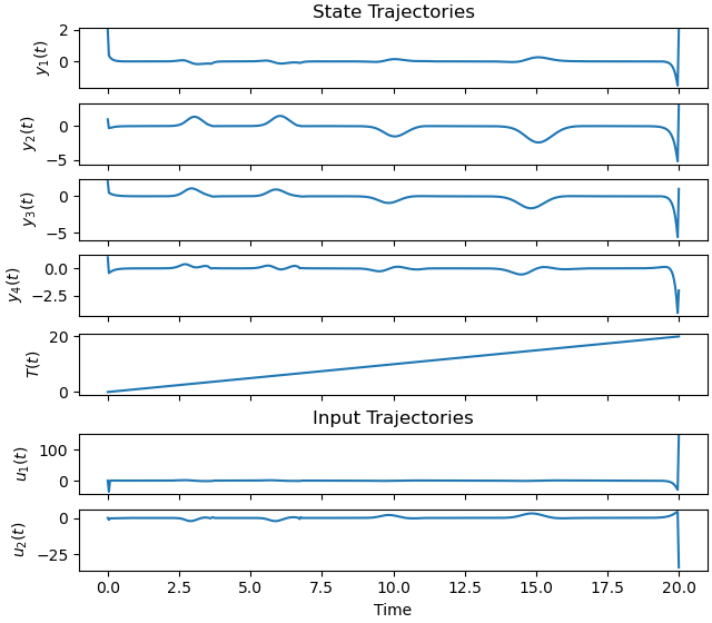
Plot the optimal state and input trajectories.

_ = prob.plot_trajectories(solution)

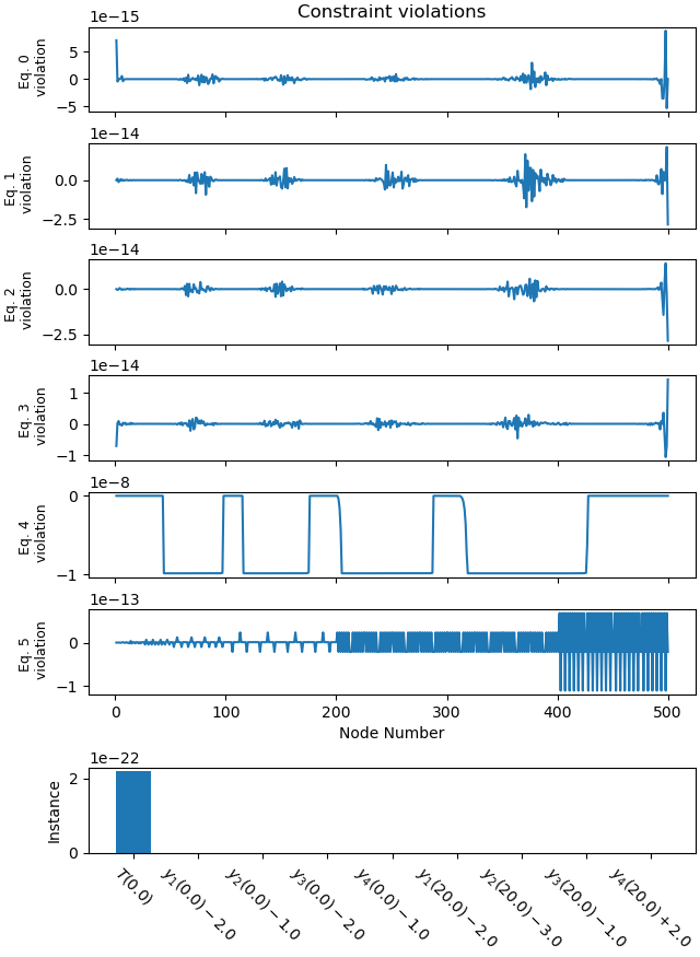
Plot the constraint violations.

_ =prob.plot_constraint_violations(solution, subplots=True)

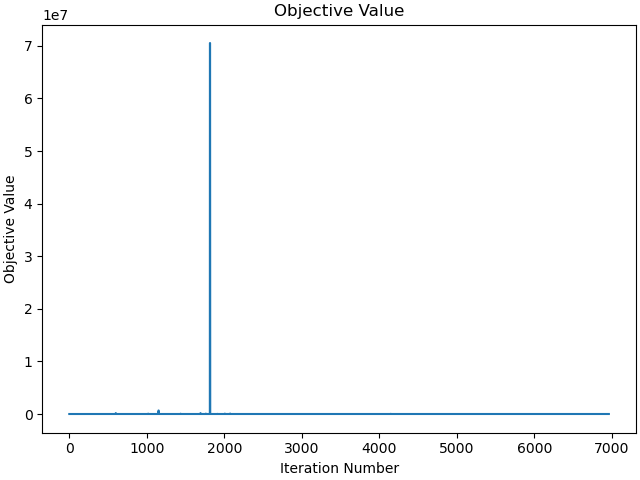
Plot the objective function as a function of optimizer iteration.

_ = prob.plot_objective_value()