Two-Strain Tuberculosis Model (betts_10_133)

This is example 10.133 from John T.Betts, Practical Methods for Optimal Control Using NonlinearProgramming, 3rd edition, Chapter 10: Test Problems.

More details may be found in chapter 8.17 of this book.

States

• \(S, T, L_1, I_1, L_", I_2\) : state variables

Controls

• \(u_1, u_2\) : control variables

import numpy as np
import sympy as sm
import sympy.physics.mechanics as me
import time
from opty import Problem
from opty.utils import create_objective_function, MathJaxRepr

Equations of Motion.

start = time.time()
t = me.dynamicsymbols._t

S, T, L1, I1, L2, I2 = me.dynamicsymbols('S T L1 I1 L2 I2')
u1, u2 = me.dynamicsymbols('u1, u2')

beta1, d2, r2, betastar, beta2, k1, p, B1, nu, k2, q, B2, d1, r1, N = \
    sm.symbols('beta1 d2 r2 betastar beta2 k1 p B1 nu k2 q B2 d1 r1 N')

Lambda = nu * N

eom = sm.Matrix([
    -S.diff(t) + Lambda - beta1*S*I1/N - betastar*S*I2/N - nu*S,
    -T.diff(t) + (u1*r1*L1 - nu*T + (1-(1-u2)*(p+q))*r2*I1 -
                  beta2*T*I1/N - betastar*T*I2/N),
    -L1.diff(t) + (beta1*S*I1/N - (nu+k1)*L1 - u1*r1*L1 +
                   (1-u2)*p*r2*I1 + beta2*T*I1/N - betastar*L1*I2/N),
    -L2.diff(t) + (1-u2)*q*r2*I1 - (nu+k2)*L2 + betastar*(S+L1+T)*I2/N,
    -I1.diff(t) + k1*L1 - (nu+d1)*I1 - r2*I1,
    -I2.diff(t) + k2*L2 - (nu+d2)*I2,
])

MathJaxRepr(eom)

$$\left[\begin{matrix}N \nu - \nu S - \dot{S} - \frac{\beta_{1} I_{1} S}{N} - \frac{betastar I_{2} S}{N}\\- \nu T + r_{1} L_{1} u_{1} + r_{2} \left(- \left(1 - u_{2}\right) \left(p + q\right) + 1\right) I_{1} - \dot{T} - \frac{\beta_{2} I_{1} T}{N} - \frac{betastar I_{2} T}{N}\\p r_{2} \left(1 - u_{2}\right) I_{1} - r_{1} L_{1} u_{1} - \left(k_{1} + \nu\right) L_{1} - \dot{L}_{1} + \frac{\beta_{1} I_{1} S}{N} + \frac{\beta_{2} I_{1} T}{N} - \frac{betastar I_{2} L_{1}}{N}\\q r_{2} \left(1 - u_{2}\right) I_{1} - \left(k_{2} + \nu\right) L_{2} - \dot{L}_{2} + \frac{betastar \left(L_{1} + S + T\right) I_{2}}{N}\\k_{1} L_{1} - r_{2} I_{1} - \left(d_{1} + \nu\right) I_{1} - \dot{I}_{1}\\k_{2} L_{2} - \left(d_{2} + \nu\right) I_{2} - \dot{I}_{2}\end{matrix}\right]$$

Define and Solve the Optimization Problem

num_nodes = 801

t0, tf = 0.0, 5.0
interval_value = tf / (num_nodes - 1)

state_symbols = (S, T, L1, L2, I1, I2)
unkonwn_input_trajectories = (u1, u2)

par_map = {
    beta1: 13,
    d2: 0.0,
    r2: 1.0,
    betastar: 0.029,
    beta2: 13,
    k1: 0.5,
    p: 0.4,
    B1: 50,
    nu: 0.0143,
    k2: 1.0,
    q: 0.1,
    B2: 500,
    d1: 0.0,
    r1: 2.0,
    N: 30000,
}

Specify the objective function and form the gradient.

objective = sm.Integral((L2 + I2 + 0.5*B1*u1**2 +
                         0.5*B2*u2**2).subs(par_map), t)

obj, obj_grad = create_objective_function(
    objective,
    state_symbols,
    unkonwn_input_trajectories,
    tuple(),
    num_nodes,
    interval_value,
)

Instance constraints and bounds.

instance_constraints = (
    S.func(t0) - 76*par_map[N]/120,
    T.func(t0) - par_map[N]/120,
    L1.func(t0) - 36*par_map[N]/120,
    I1.func(t0) - 4*par_map[N]/120,
    L2.func(t0) - 2*par_map[N]/120,
    I2.func(t0) - par_map[N]/120,
)

bounds = {
        u1: (0.05, 0.95),
        u2: (0.05, 0.95),
}

Create the optimization problem.

prob = Problem(
    obj,
    obj_grad,
    eom,
    state_symbols,
    num_nodes,
    interval_value,
    instance_constraints=instance_constraints,
    known_parameter_map=par_map,
    bounds=bounds,
    time_symbol=t,
    )

Acceptable tolerance and iteration settings are lowered, to get convergence with a reasonable number of iterations.

prob.add_option('max_iter', 4000)
prob.add_option('acceptable_tol', 1e-2)
prob.add_option('acceptable_iter', 5)

Rough initial guess.

initial_guess = np.ones(prob.num_free)

Find the optimal solution.

start_solve = time.time()
solution, info = prob.solve(initial_guess)
end_solve = time.time()
print(f"Solve time: {end_solve - start_solve:.3f} seconds")

print(info['status_msg'])
Jstar = 5152.07310
print(f"Objective value achieved: {info['obj_val']:.4f}, ",
      f"as per the book it is {Jstar:.4f}, so the deviation is: ",
      f"{(info['obj_val'] - Jstar) / Jstar*100:.3f} %")
Tbstar = 1123
print(f"Individuals infected with resistant Tb = ",
      f"{solution[4*num_nodes-1] + solution[6*num_nodes-1]:.3f}, ",
      f"vs. {Tbstar} from the book, hence deviation: ",
      f"{(solution[4*num_nodes-1] + solution[6*num_nodes-1] -
         Tbstar) / Tbstar*100:.3f} %")

Solve time: 65.949 seconds
b'Algorithm stopped at a point that was converged, not to "desired" tolerances, but to "acceptable" tolerances (see the acceptable-... options).'
Objective value achieved: 5154.9859,  as per the book it is 5152.0731, so the deviation is:  0.057 %
Individuals infected with resistant Tb =  1121.198,  vs. 1123 from the book, hence deviation:  -0.160 %

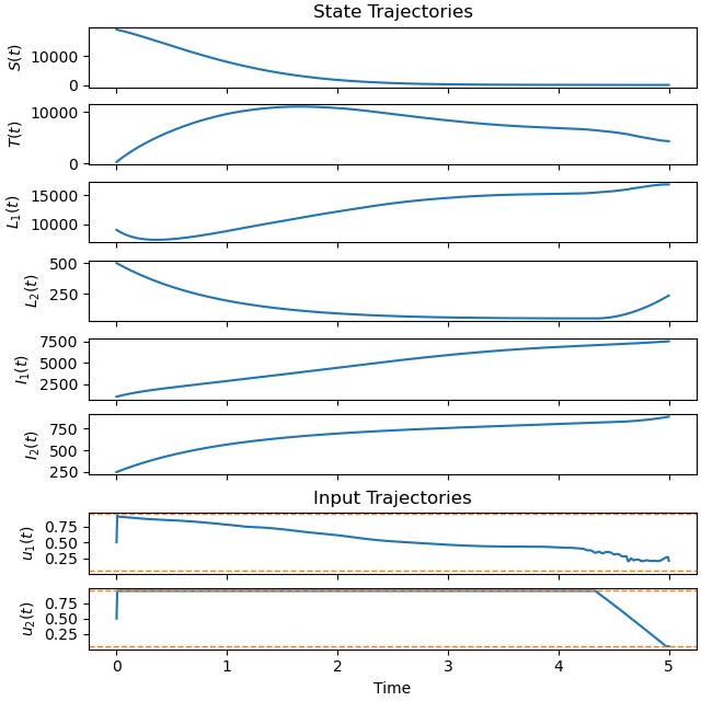
Plot the optimal state and input trajectories.

_ = prob.plot_trajectories(solution, show_bounds=True)

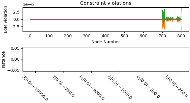
Plot the constraint violations.

_ = prob.plot_constraint_violations(solution)

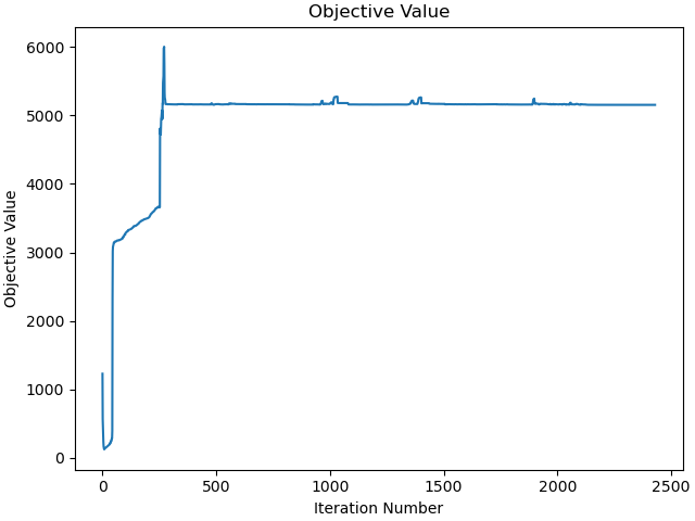
Plot the objective function as a function of optimizer iteration.

_ = prob.plot_objective_value()