Note
Go to the end to download the full example code.
Ball bouncing between two planes
Objective
Show how to use tow methods of impact forces to at least qualitatively simulate an experiment
Description
An elastic homogenious ball of radius r and mass m is bouncing between two horizontal planes, one being at z = 0, the other one at z = H. Essentially I want to simulate the simplest example of this video:
https://www.youtube.com/watch?v=g_VxOIlg7q8
An observer (a particle) of mass \(m_o\) may be put anywhere inside the ball. Gravitiy points in the negative Z direction.
Notes
First I tried a friction model, where the force to change \(\omega\) is friction, depending on the vertical impact force and a coefficient of \(\mu\). I easily found parameters to stop the advancing of the ball, but I could not reverse it, like shown in the video.
Then I tried a dig in model, where the ball does not slide at all, the impact force is in the direction of the speed of the contact point. This surely made the ball reverse its direction, but unrealistically so, I thought. Also some other issues
So, I mixed the two models, like: force on the ball = (1 - mixtur) \(\cdot\) force of friction model + mixtur \(\cdot\) force of no slip model. With mixtur \(\approx\) 0.35 this gave reasonable results. Maybe this really describes reality to some extend, I know too little about realistic impacts.
The animation may be made smoother by increasing
zeitpunktebelow.
Variables, Parameters
\(N\): inertial frame, fixed in space
\(A\): frame fixed to the ball
\(O\): point fixed in N, the origin of the inertial frame
\(Dmc\): center of the ball, a RigidBody
\(P_o\): the observer, a Particle
\(BCP_u, BCP_o\): corresponding points fixed on the ball, the contact points with the lower and upper plane respectively
\(q_1, q_2, q_3\): angles of the ball w.r.t. N
\(u_1, u_2, u_3\): angular velocities of the ball
\(m_1, m_2, m_3\): location of the center of the ball, relative to the inertial frame N
\(um_1, um_2, um_3\): the speeds of the center of the ball
\(c_{tau}\): the experimental constant needed for Hunt-Crossley
\(\mu\): the friction constant
\(ny_b, ny_p\): Poisson’s ratio of ball and plane respectively.
\(E_b, E_p\): Young’s modulus of ball and plane respectively
\(rhodt_{u}\): speed right before the impact with the lower plane
\(rhodt_{o}\): speed right before the impact with the upper plane
\(m, m_o, i_{XX}, i_{YY}, i_{ZZ}\): mass of ball, mass of observer, moments of inertia of the ball
\(\alpha, \beta, \gamma\): describe the location of the observer relative to the center of the ball
\(ru_1, ru_2, ru_3\): See explanation below.
\(ro_1, ro_2, ro_3\): See explanation below.
\(\textrm{mixtur}\): See explanation above.
\(H\): height of the upper plane
import sympy as sm
import sympy.physics.mechanics as me
import numpy as np
import matplotlib.pyplot as plt
import matplotlib as mp
from matplotlib.animation import FuncAnimation
from scipy.integrate import solve_ivp
mp.rcParams['animation.embed_limit'] = 2**128
# Kane's Equations of Motion
# --------------------------
t = me.dynamicsymbols._t
N, A = sm.symbols('N, A', cls=me.ReferenceFrame)
O, Dmc, Po, BCPu, BCPo = sm.symbols('O, Dmc, Po, BCPu, BCPo', cls=me.Point)
q1, q2, q3, u1, u2, u3 = me.dynamicsymbols('q1, q2, q3, u1, u2, u3')
m1, m2, m3, um1, um2, um3 = me.dynamicsymbols('m1, m2, m3, um1, um2, um3')
m, mo, g, r, alpha, beta, gamma, iXX, iYY, iZZ, H = sm.symbols('m, mo, g, r, '
'alpha, beta, '
'gamma, iXX, '
'iYY, iZZ, H')
nyb, nyp, Eb, Ep, rhodtu, rhodto, ctau, mu = sm.symbols('nyb, nyp, Eb, Ep, '
'rhodtu, rhodto, ctau,'
' mu')
ru1, ru2, ru3, ro1, ro2, ro3 = sm.symbols('ru1, ru2, ru3, ro1, ro2, ro3')
mixtur = sm.symbols('mixtur')
A.orient_body_fixed(N, (q1, q2, q3), '123')
rot = A.ang_vel_in(N)
A.set_ang_vel(N, u1*N.x + u2*N.y + u3*N.z)
rot1 = A.ang_vel_in(N)
O.set_vel(N, 0)
Dmc.set_pos(O, m1*N.x + m2*N.y + m3*N.z)
Dmc.set_vel(N, um1*N.x + um2*N.y + um3*N.z)
Po.set_pos(Dmc, r * (alpha*A.x + beta*A.y + gamma*A.z))
_ = Po.v2pt_theory(Dmc, N, A)
Points of impact
The potential contact points of the ball with the plane are obviously these: \(BCP_u(m_1 / m_2 / -r)\) and \(CP_o(m_1, m_2, r)\)
BCPu.set_pos(Dmc, -r*N.z)
BCPu.v2pt_theory(Dmc, N, A)
BCPo.set_pos(Dmc, r*N.z)
BCPo.v2pt_theory(Dmc, N, A)
(r*u2(t) + um1(t))*N.x + (-r*u1(t) + um2(t))*N.y + um3(t)*N.z
Function which calculates the forces of an impact between the ball and the horizontal planes for the friction model
The impact force is on the line normal to the plane, that is in Z direction, and goes through the center of the ball, \(Dmc\). I use Hunt Crossley’s method to calculate it.
The impact force is on the line normal to the plane, that is in Z direction, and goes through the center of the ball, \(Dmc\). I use Hunt Crossley’s method to calculate it. It’s direction points from the plane to the ball.
The friction force acting on the contact point \(BCP_u\) is in the direction of the component of \(\dfrac{d}{dt} BCP_u\) in the plane. It’s magnitude is the impact force times a friction factor \(m_{uW}\). (Of course same for the upper contact point \(BCP_o\))
Note about the force during the collisions
Hunt Crossley’s method
My reference is this article: https://www.sciencedirect.com/science/article/pii/S0094114X23000782
This is with dissipation during the collision, the general force is given in (63) as \(f_n = k_0 \cdot \rho + \chi \cdot \dot \rho\), with \(k_0\) as above, \(\rho\) the penetration, and \(\dot\rho\) the speed of the penetration.
In the article it is stated, that \(n = \frac{3}{2}\) is a good choice, it is derived in Hertz’ approach. Of course, \(\rho, \dot\rho\) must be the signed magnitudes of the respective vectors.
A more realistic force is given in (64) as:
\(f_n = k_0 \cdot \rho^n + \chi \cdot \rho^n\cdot \dot \rho\), as this avoids discontinuity at the moment of impact.
Hunt and Crossley give this value for \(\chi\), see table 1:
\(\chi = \dfrac{3}{2} \cdot(1 - c_\tau) \cdot \dfrac{k_0}{\dot \rho^{(-)}}\),
where
\(c_\tau = \dfrac{v_1^{(+)} - v_2^{(+)}}{v_1^{(-)} - v_2^{(-)}}\),
where \(v_i^{(-)}, v_i^{(+)}\) are the speeds of \(body_i\), before and after the collosion, see (45),
\(\dot\rho^{(-)}\) is the speed right at the time the impact starts.
\(c_\tau\) is an experimental factor, apparently around 0.8 for steel.
Using (64), this results in their expression for the force:
\(f_n = k_0 \cdot \rho^n \left[1 + \dfrac{3}{2} \cdot(1 - c_\tau) \cdot \dfrac{\dot\rho}{\dot\rho^{(-)}}\right]\)
with
\(k_0 = \frac{4}{3\cdot(\sigma_1 + \sigma_2)} \cdot \sqrt{\frac{R_1 \cdot R_2}{R_1 + R_2}}\), where \(\sigma_i = \frac{1 - \nu_i^2}{E_i}\),
with
\(\nu_i\) = Poisson’s ratio, \(E_i\) = Young’s modulus, \(R_1, R_2\) the radii of the colliding bodies, \(\rho\) the penetration depth. All is near equations (54) and (61) of this article.
For the plane, I set \(R_2 = \infty\), so \(k_0\) simplifies to \(k_0 = \frac{4}{3\cdot(\sigma_1 + \sigma_2)} \cdot \sqrt{R_1}\),
with
\(R_1 = r\), the radius of the ball. I am not sure, this is covered by the theory.
As per the article, \(n = \frac{3}{2}\) is always to be used, I believe, Hertz derived this on theoretical grounds.
spring energy = \(k_0 \cdot \int_{0}^{\rho} k^{3/2}\,dk = k_0 \cdot\frac{2}{5} \cdot \rho^{5/2}\)
I assume, the dissipated energy cannot be given in closed form, at least the article does not give one.
Note
\(c_\tau = 1.\) gives Hertz’s solution to the impact problem, also described in the article.
Friction when the ball hits the street
If \(\dfrac{d}{dt} BCP_u\) ist the speed of the contact point of the ball with the plane, then \(\left[\dfrac{d}{dt} BCP_u - \left( \dfrac{d}{dt} BCP_u \circ N.z \right) \cdot N.z \right]\) is the speed component in the plane.
As there are numerical problems when \(\left| \left[\dfrac{d}{dt} BCP_u - \left( \dfrac{d}{dt} BCP_u \circ N.z \right) \cdot N.z \right] \right| \approx 0\), I use \(\left| \left[\dfrac{d}{dt} BCP_u - \left( \dfrac{d}{dt} BCP_u \circ N.z \right) \cdot N.z \right] \right| \vee 10^{-10}\).
def fric_lower_plane(rhodtu):
# force acting on BCPu
# should always be positive, the ball must not fall through the planes
abstand = m3
# pointing towards the ball
richtung = N.z
# positive in the ball has penetrated the plane
rho = r - abstand
# speed of the contact point of the ball
vCP = BCPu.vel(N)
# speed component in Z direction pointing from the ball to the plane
rhodt = me.dot(vCP, richtung)
rho = sm.Abs(rho)
# determine k0
wurzel = sm.sqrt(r)
sigma_b = (1. - nyb**2) / Eb
sigma_s = (1. - nyp**2) / Ep
k0 = 4. / (3.*(sigma_b + sigma_s)) * wurzel
# Impact force on BCPu in Z direction
# Here I assume, that the penetration is small, otherwise I would not know
# how to do it.
forcec = (k0 * rho**(3/2) * (1. + 3./2. * (1 - ctau) * (-rhodt) /
sm.Abs(rhodtu)) * richtung *
sm.Heaviside(r - abstand, 0.))
# The speed component of vCP in the plane is, of course, the speed minus
# its component perpendicular to the plane.
vx = vCP - (me.dot(vCP, richtung)) * richtung
# Here, Heaviside probably not really needed.
forcef = (forcec.magnitude() * mu * (-vx) * sm.Heaviside(r - abstand, 0.) *
1. / sm.Max(vx.magnitude(), 1.e-10))
# The force acting on BCPu is returned
return forcec + forcef
Same comments as above.
def fric_upper_plane(rhodto):
# force acting on BCPo
# should always be positive, the ball must not fall through the planes
abstand = H - m3
# pointing towards the ball
richtung = -N.z
# positive in the ball has penetrated the plane
rho = r - abstand
# speed of the contact point of the ball
vCP = BCPo.vel(N)
# speed component in Z direction pointing from the ball to the plane
rhodt = me.dot(vCP, richtung)
rho = sm.Abs(rho)
# determine k0
wurzel = sm.sqrt(r)
sigma_b = (1. - nyb**2) / Eb
sigma_s = (1. - nyp**2) / Ep
k0 = 4. / (3.*(sigma_b + sigma_s)) * wurzel
# Impact force on BCP0 in Z direction
# Here I assume, that the penetration is small, otherwise I would not know
# how to do it.
forcec = (k0 * rho**(3/2) * (1. + 3./2. * (1 - ctau) * (-rhodt) /
sm.Abs(rhodto)) * richtung *
sm.Heaviside(r - abstand, 0.))
# The speed component of vCP in the plane is, of course, the speed minus
# its component perpendicular to the plan.
vx = vCP - (me.dot(vCP, richtung)) * richtung
forcef = (forcec.magnitude() * mu * (-vx) * sm.Heaviside(r - abstand, 0.) *
1./sm.Max(vx.magnitude(), 1.e-10))
# The force acting on BCPu is returned
return forcec + forcef
Here I assume, that the ball does not slide on the plane when it hits it, but ‘digs into the plane’ in the direction of the speed of the contact point. I do not know, whether this is covered by the Hunt-Crossley theory, which I use to calculate the impact forces.
As there are numerical problems when \(\left| \dfrac{d}{dt} BCP_u \right| \approx 0\), I calculate \(\dfrac{d}{dt} BCP_u\) right before the impact during the integration, and hand \(ru_1, ru_2, ru_3\) to the function,
where:
\(\dfrac{d}{dt} BCP_u = ru_1 \cdot N.x + ru_2 \cdot N.y + ru_3 \cdot N.z\) As the duration of the impact is short, I do not think, the error caused by this simplification (keeping the direction of the force constant during impact) has much effect.
def HC_lower_plane(rhodtu, ru1, ru2, ru3):
# force acting on BCPu
# should always be positive, the ball must not fall through the planes
abstand = m3
# speed of the contact point on the ball
vCP = BCPu.vel(N)
# pointing towards the ball. To be consistent, I want this to be a unit
# vector, and always point towards the ball
richtung = -(ru1*N.x + ru2*N.y + ru3*N.z)
# positive in the ball has penetrated the plane
rho = r - abstand
# speed component in Z direction pointing from the ball to the plane
rhodt = me.dot(vCP, richtung)
rho = sm.Abs(rho)
# determine k0
wurzel = sm.sqrt(r)
sigma_b = (1. - nyb**2) / Eb
sigma_p = (1. - nyp**2) / Ep
k0 = 4. / (3.*(sigma_b + sigma_p)) * wurzel
# Impact force on BCPu
# Here I assume, that the penetration is small, otherwise I would not know
# how to do it.
forcec = (k0 * rho**(3/2) * (1. + 3./2. * (1 - ctau) * (-rhodt) /
sm.Abs(rhodtu)) * richtung *
sm.Heaviside(r - abstand, 0.))
# The force acting on BCPu is returned
return forcec
Collision with the upper plane. Same comments as above.
def HC_upper_plane(rhodto, ro1, ro2, ro3):
# force acting on BCPo
abstand = H - m3
vCP = BCPo.vel(N)
richtung = -(ro1*N.x + ro2*N.y + ro3*N.z)
rho = r - abstand
rhodt = me.dot(vCP, richtung)
rho = sm.Abs(rho)
# determine k0
wurzel = sm.sqrt(r)
sigma_b = (1. - nyb**2) / Eb
sigma_s = (1. - nyp**2) / Ep
k0 = 4. / (3.*(sigma_b + sigma_s)) * wurzel
# Impact force on BCPo
forcec = (k0 * rho**(3/2) * (1. + 3./2. * (1 - ctau) * (-rhodt) /
sm.Abs(rhodto)) * richtung *
sm.Heaviside(r - abstand, 0.))
# The force acting on BCPu is returned
return forcec
Kane’s equations.
Ib = me.inertia(A, iXX, iYY, iZZ)
body = me.RigidBody('body', Dmc, A, m, (Ib, Dmc))
Poa = me.Particle('Poa', Po, mo)
BODY = [body, Poa]
F1f = [(Dmc, -m*g*N.z), (Po, -mo*g*N.z)]
F2f = [(BCPu, (sm.S(1.) - mixtur) * fric_lower_plane(rhodtu))]
F3f = [(BCPo, (sm.S(1.) - mixtur) * fric_upper_plane(rhodto))]
F1hc = [(Dmc, -m*g*N.z), (Po, -mo*g*N.z)]
F2hc = [(BCPu, mixtur * HC_lower_plane(rhodtu, ru1, ru2, ru3))]
F3hc = [(BCPo, mixtur * HC_upper_plane(rhodto, ro1, ro2, ro3))]
FL = (F1f + F2f + F3f) + (F2hc + F3hc)
q_ind = [q1, q2, q3] + [m1, m2, m3]
u_ind = [u1, u2, u3] + [um1, um2, um3]
kd = [me.dot(rot - rot1, uv) for uv in A] + [i - j.diff(t)
for i, j in zip((um1, um2, um3),
(m1, m2, m3))]
KM = me.KanesMethod(N, q_ind=q_ind, u_ind=u_ind, kd_eqs=kd)
(fr, frstar) = KM.kanes_equations(BODY, FL)
MM = KM.mass_matrix_full
force = KM.forcing_full
print(f'force has {sm.count_ops(force):,} operations')
print(f'MM has {sm.count_ops(MM):,} operations')
force has 60,602 operations
MM has 3,337 operations
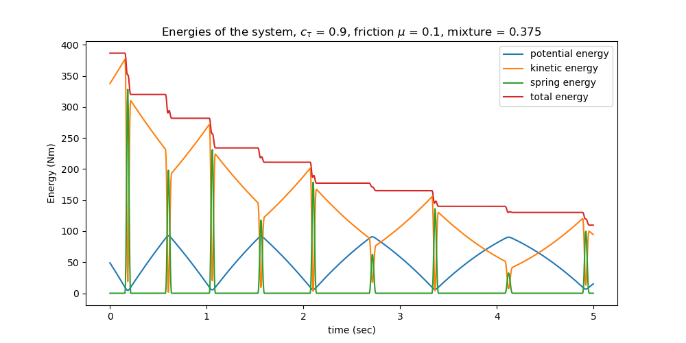
I like to look at the energies of the system. This has often told me I had made a mistake in the equations of motion. So, these functions are defined here.
pot_energie = (m * g * me.dot(Dmc.pos_from(O), N.z) + mo * g *
me.dot(Po.pos_from(O), N.z))
kin_energie = sum([koerper.kinetic_energy(N) for koerper in BODY])
rho1 = r - m3 # positive if impact with lower plane
rho2 = r - (H - m3) # positive if impact with upper plane
sigma_b = (1. - nyb**2) / Eb
sigma_p = (1. - nyp**2) / Ep
k0 = 4. / (3.*(sigma_b + sigma_p)) * sm.sqrt(r)
spring_energie = (2. / 5. * k0 * sm.Abs(rho1)**(5 / 2) *
sm.Heaviside(rho1, 0.) + 2. / 5. * k0 *
sm.Abs(rho2)**(5 / 2) * sm.Heaviside(rho2, 0.))
# speed of BCPu in direction of the lower plane
rhodtuu = me.dot(BCPu.vel(N), -N.z)
rhodtoo = me.dot(BCPo.vel(N), N.z) # analoguously dto.
Lambdification
qL = q_ind + u_ind
pL1 = [m, mo, g, r, alpha, beta, gamma, iXX, iYY, iZZ, H, mixtur]
pL2 = [nyb, nyp, Eb, Ep, ctau, mu, rhodtu, rhodto, ru1, ru2, ru3, ro1,
ro2, ro3]
pL = pL1 + pL2
MM_lam = sm.lambdify(qL + pL, MM, cse=True)
force_lam = sm.lambdify(qL + pL, force, cse=True)
pot_lam = sm.lambdify(qL + pL, pot_energie, cse=True)
kin_lam = sm.lambdify(qL + pL, kin_energie, cse=True)
spring_lam = sm.lambdify(qL + pL, spring_energie, cse=True)
rhodtu_lam = sm.lambdify(qL + pL, rhodtuu, cse=True)
rhodto_lam = sm.lambdify(qL + pL, rhodtoo, cse=True)
richtungu_lam = sm.lambdify(qL + pL, [me.dot(BCPu.vel(N).normalize(), uv)
for uv in N], cse=True)
richtungo_lam = sm.lambdify(qL + pL, [me.dot(BCPo.vel(N).normalize(), uv)
for uv in N], cse=True)
The parameters and the initial conditions are set here. For their meaning, see above.
# Set parameters and initial conditions.
mixtur1 = 0.375
m11, m21, m31 = 0., 0., 5.
um11, um21, um31 = -5., 5., -25.
q11, q21, q31 = 0., 0., 0.
u11, u21, u31 = 0., 0., 0.
mb1 = 1.
mo1 = 0.0001
r1 = 1.
H1 = 10.
nyb1 = 0.25 # Poisson's ratio for rubber, from the internet
nyp1 = 0.15 # Poisson's ratio for concrete, from the internet
Eb1 = 3.e3 # Young's modulus for rubber is really about 3.e9
Ep1 = 2.e10 # Young's modulus for steel is really about 2.e11
ctau1 = 0.90 # experimental constant
mu1 = 0.1 # coefficient of friction
alpha1, beta1, gamma1 = 0.7, 0., 0.7
intervall = 5.0
rhodtu1, rhodto1 = 1., 1. # of no importance here.any value o.k.
ru11, ru21, ru31, ro11, ro21, ro31 = 1., 1., 1., 1., 1., 1. # dto.
if alpha1**2 + beta1**2 + gamma1**2 >= 1.:
raise Exception('Observer is outside of the ball')
schritte = int(intervall * 1000.) # this should be slightly less than nfev
iXX1 = 2. / 5. * mb1 * r1**2 # from the internet.
iYY1 = iXX1
iZZ1 = iXX1
pL_vals1 = [mb1, mo1, 9.81, r1, alpha1, beta1, gamma1, iXX1, iYY1, iZZ1,
H1, mixtur1]
pL_vals2 = [nyb1, nyp1, Eb1, Ep1, ctau1, mu1, rhodtu1, rhodto1, ru11, ru21,
ru31, ro11, ro21, ro31]
pL_vals = pL_vals1 + pL_vals2
y0 = [q11, q21, q31, m11, m21, m31] + [u11, u21, u31, um11, um21, um31]
Numerical Integration
The parameters \(rhodt_u, rhodt_o, ru_1, ru_2, ru_3, ro_1, ro_2, ro_3\) are available only during integration, but needed later for the Energy. So, I collect them during integration.
times = np.linspace(0, intervall, schritte)
t_span = (0., intervall)
impact_list = []
# I try to reduce the number of entries into the impact_list.
# Not really essential.
zaehler = 0
zeit_list = []
params_list = []
def gradient(t, y, args):
global zaehler
# set rhodtu / rhodto
if r1 < y[5] < r1 + 0.01:
zaehler += 1
args[-8] = rhodtu_lam(*y, *args)
if zaehler == 1:
impact_list.append([t, y[3], y[4], y[5]])
tu1, tu2, tu3 = richtungu_lam(*y, *args)
# I want the speed vector only when the ball moves into the plane,
# not when it moves out. this would give the wrong direction.
if tu3 < 0.:
args[-6], args[-5], args[-4] = tu1, tu2, tu3
elif r1 < H1 - y[5] < r1 + 0.01:
zaehler += 1
args[-7] = rhodto_lam(*y, *args)
if zaehler == 1:
impact_list.append([t, y[3], y[4], y[5]])
to1, to2, to3 = richtungo_lam(*y, *args)
# Same idea as above.
if to3 > 0.:
args[-3], args[-2], args[-1] = to1, to2, to3
else:
zaehler = 0
zeit_list.append(t)
params_list.append(args)
sol = np.linalg.solve(MM_lam(*y, *args), force_lam(*y, *args))
return np.array(sol).T[0]
resultat1 = solve_ivp(gradient, t_span, y0, t_eval=times, args=(pL_vals,),
atol=1.e-12, rtol=1.e-12, method='Radau')
resultat = resultat1.y.T
print('resultat shape', resultat.shape, '\n')
print(resultat1.message, '\n')
print(f'To numerically integrate an intervall of {intervall} sec the routine '
f' cycled {resultat1.nfev:,} times.')
resultat shape (5000, 12)
The solver successfully reached the end of the integration interval.
To numerically integrate an intervall of 5.0 sec the routine cycled 151,645 times.
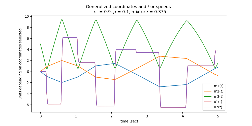
Plot any generalized coordinates or speeds you want to see. I consider around zeitpunkte points in time.
# reduce the number of points of time to around zeitpunkte
times2 = []
resultat2 = []
index2 = []
zeitpunkte = 1000
reduction = max(1, int(len(times)/zeitpunkte))
for i in range(len(times)):
if i % reduction == 0:
times2.append(times[i])
resultat2. append(resultat[i])
schritte2 = len(times2)
resultat2 = np.array(resultat2)
times2 = np.array(times2)
test = '$c_{\\tau}$'
bezeichnung = [str(i) for i in qL]
fig, ax = plt.subplots(figsize=(10, 5))
for i in (3, 4, 5, 6, 7):
ax.plot(times2, resultat2[:, i], label=bezeichnung[i])
ax.set_xlabel('time (sec)')
ax.set_ylabel('units depending on coordinates selected')
_ = ax.set_title((f'Generalized coordinates and / or speeds \n {test} = '
f'{ctau1}. $\\mu$ = {mu1}, mixture = {mixtur1}'))
_ = ax.legend()
Plot the energies of the system.
The parameters \(rhodt_u, rhodt_o, ru_1, ru_2, ru_3, ro_1, ro_2, ro_3\) were collected at each step of the integration because they are needed here. I try to match the times when they were collected closely to the times returned at the end of the integration.
argumente = [0]
zeitw = np.array(zeit_list)
for zeit1 in times[: -1]:
start = argumente[-1]
start1 = np.min(np.argwhere(zeitw >= zeit1))
argumente.append(start1)
if len(argumente) != len(times):
raise Exception('Something went wrong')
pot_np = np.empty(resultat2.shape[0])
kin_np = np.empty(resultat2.shape[0])
spring_np = np.empty(resultat2.shape[0])
total_np = np.empty(resultat2.shape[0])
for i in range(schritte2):
pL_vals = params_list[argumente[i]]
pot_np[i] = pot_lam(*resultat2[i, :], *pL_vals)
kin_np[i] = kin_lam(*resultat2[i, :], *pL_vals)
spring_np[i] = spring_lam(*resultat2[i, :], *pL_vals)
total_np[i] = pot_np[i] + kin_np[i] + spring_np[i]
fig, ax = plt.subplots(figsize=(10, 5))
ax.plot(times2, pot_np, label='potential energy')
ax.plot(times2, kin_np, label='kinetic energy')
ax.plot(times2, spring_np, label='spring energy')
ax.plot(times2, total_np, label='total energy')
ax.set_xlabel('time (sec)')
ax.set_ylabel('Energy (Nm)')
test = '$c_{\\tau}$'
ax.set_title((f'Energies of the system, {test} = {ctau1}, friction $\\mu$ ='
f' {mu1}, mixture = {mixtur1}'))
_ = ax.legend()
Animation
zeitpunkte = 90
times2 = []
resultat2 = []
index2 = []
reduction = max(1, int(len(times)/zeitpunkte))
for i in range(len(times)):
if i % reduction == 0:
times2.append(times[i])
resultat2.append(resultat[i])
schritte2 = len(times2)
print(f'animation used {schritte2} points in time')
resultat2 = np.array(resultat2)
times2 = np.array(times2)
# location of particle
Po_loc = [me.dot(Po.pos_from(O), uv) for uv in N]
Po_loc_lam = sm.lambdify(qL + pL, Po_loc, cse=True)
Pox, Poy, Poz = Po_loc_lam(*[resultat2[:, j]
for j in range(resultat.shape[1])], *pL_vals)
# Get only one contact point for each impact. I assume, that subsequent
# impacts have a time difference of at least 0.1 sec.
impact_net = []
impact_net.append(impact_list[0])
zeit1 = impact_net[0][0]
for i in range(len(impact_list)):
if impact_list[i][0] - zeit1 < 0.1:
pass
else:
zeit1 = impact_list[i][0]
impact_net.append(impact_list[i])
print('Number of contact points detected', len(impact_net))
# plot the horizontal plane H
def plot_3d_plane(x_min, x_max, y_min, y_max, z_wert, alpha1):
# Create a meshgrid for x and y values
x = np.linspace(x_min, x_max, 100)
y = np.linspace(y_min, y_max, 100)
x, y = np.meshgrid(x, y)
# Z values are set to 0 for the plane
z = np.ones_like(x) * z_wert
# Plot the 3D plane
ax.plot_surface(x, y, z, alpha=alpha1, rstride=100, cstride=100, color='c')
# Function to create ellipsoid points
def create_ellipsoid(a, b, c, theta, phi, delta, offset):
u = np.linspace(0, 2 * np.pi, 20)
v = np.linspace(0, np.pi, 20)
x = a * np.outer(np.cos(u), np.sin(v))
y = b * np.outer(np.sin(u), np.sin(v))
z = c * np.outer(np.ones(np.size(u)), np.cos(v))
# Rotation matrix
# rotation around Z axis
R_theta = np.array([[np.cos(theta), -np.sin(theta), 0],
[np.sin(theta), np.cos(theta), 0],
[0, 0, 1]])
# rotation around Y axis
R_phi = np.array([[np.cos(phi), 0, np.sin(phi)],
[0, 1, 0],
[-np.sin(phi), 0, np.cos(phi)]])
# rotation around X axis
R_delta = np.array([[1, 0, 0],
[0, np.cos(delta), -np.sin(delta)],
[0, np.sin(delta), np.cos(delta)]])
rotated_coords = (np.dot(np.dot(np.dot(
np.array([x.flatten(), y.flatten(), z.flatten()]).T, R_theta), R_phi),
R_delta).T)
rotated_coords1 = rotated_coords.reshape(3, 20, 20)
for i in range(20):
for j in range(20):
rotated_coords1[:, i, j] = (rotated_coords1[:, i, j] +
np.array([offset[0], offset[1],
offset[2]]))
return rotated_coords1
maxx = np.max(resultat2[:, 3])
minx = np.min(resultat2[:, 3])
maxy = np.max(resultat2[:, 4])
miny = np.min(resultat2[:, 4])
maxx = max(maxx, maxy) + 1.
minx = min(minx, miny) - 1
maxy = maxx
miny = minx
maxz = H1 + 1.
minz = -1.
maxmax = max(maxx, maxz)
minmin = min(minx, minz)
# This is to asign colors of 'plasma' to the impact points.
Test = mp.colors.Normalize(0, len(impact_net))
Farbe = mp.cm.ScalarMappable(Test, cmap='plasma')
# Function to update the plot in the animation
def update(frame):
plt.cla()
ax.set_xlim([minmin, maxmax])
ax.set_ylim([minmin, maxmax])
ax.set_zlim([minmin, maxmax])
message = (f'running time {times2[frame]:.2f} sec \n The red dot is the '
f'particle $P_O$ \n The lighter the color of the contact '
f'point, the later in time it happened')
ax.set_title(message, fontsize=12)
ax.set_xlabel('X direction', fontsize=12)
ax.set_ylabel('Y direction', fontsize=12)
ax.set_zlabel('Z direction', fontsize=12)
# plot lower plane
plot_3d_plane(minmin, maxmax, minmin, maxmax, 0., alpha1=0.2)
# plot upper plane
plot_3d_plane(minmin, maxmax, minmin, maxmax, H1, alpha1=0.1)
# plot the particle
ax.plot([Pox[frame]], [Poy[frame]], Poz[frame], marker='o', color='red')
impact_X = []
impact_Y = []
impact_Z = []
for i in range(len(impact_net)):
if times2[frame] > impact_net[i][0]:
impact_X.append(impact_net[i][1])
impact_Y.append(impact_net[i][2])
impact_Z.append(impact_net[i][3])
farbe2 = Farbe.to_rgba(i)
ax.plot([impact_net[i][1]], [impact_net[i][2]], [impact_net[i][3]],
marker='o', color=farbe2)
delta, phi, theta = resultat2[frame, 0: 3]
offset = [resultat2[frame, 3], resultat2[frame, 4], resultat2[frame, 5]]
ellipsoid = create_ellipsoid(r1, r1, r1, delta, phi, theta, offset)
ax.plot(impact_X, impact_Y, impact_Z, lw=0.5, color='green',
linestyle='--')
ax.plot_wireframe(ellipsoid[0], ellipsoid[1], ellipsoid[2], color='b',
alpha=0.6, lw=0.25)
# Draw arrows between impact points.
if len(impact_X) > 0:
np.random.seed(42) # For reproducibility
variation = [np.random.rand() for _ in range(len(impact_X) - 1)]
for i in range(len(impact_X) - 1):
p1 = np.array([impact_X[i], impact_Y[i], impact_Z[i]])
p2 = np.array([impact_X[i + 1], impact_Y[i + 1], impact_Z[i + 1]])
variation1 = variation[i]
midpoint = p1 * (1 - variation1) + p2 * variation1
direction = (p2 - p1) / np.linalg.norm(p2 - p1)
arrow_length = 0.25
ax.quiver(midpoint[0], midpoint[1], midpoint[2],
direction[0], direction[1], direction[2],
length=arrow_length, color='red', linewidth=2,
arrow_length_ratio=3.0)
# Create a Matplotlib figure and axis
fig = plt.figure(figsize=(10, 10))
ax = fig.add_subplot(111, projection='3d')
ax.view_init(elev=30, azim=30, roll=0.)
# Create the animation
ani = FuncAnimation(fig, update, frames=schritte2,
interval=3000*np.max(times2) / schritte2)
plt.show()