Time Delay Estimation

Objectives

• Show how a time delay in a driving force of a mechanical system may be estimated from noisy measurements by introducing a state variable which mimicks the time.

• Show how to handle the explicit appearance of the time t in the equations of motion.

• Show how to handle non-contiguous measurements.

Introduction

A simple pendulum is driven by a torque of the form: \(F \cdot t \cdot \sin(\omega (t - \delta))\), and \(F, \omega, \delta\) are to be erstimated based on noisy measurements of the angle.

Presently, opty cannot handle expressions like \(\sin(\omega \cdot (t - \delta))\) in the equations of motion. To overcome this, a state variable T(t) is introduced, \(\dfrac{dT}{dt} = 1\) is added to the equations of motion, and \(T(t_0) = t_0\) is added as a constraint. This way, T(t) and t have the same values. opty can handle \(\sin(T(t) - \delta)\) in the equations of motion without any problems.

Presently, opty cannot handle the explicit appearance of the time t in the equations of motion. To overcome this, the time t is replaced by the T(t) state variable described above.

The driving force is set to zero for \(t < \delta\).

The idea of using non-contiguous measurements was taken from this simulation:

https://github.com/csu-hmc/opty/blob/master/examples-gallery/intermediate/plot_non_contiguous_parameter_identification.py

Also the detailed explanation may be found there

Notes

• It is helpful to give reasonable bounds for the parameters to be estimated. Otherwise opty may converge to another local minimum.

• If the initial speeds \(u_i \neq 0\), it seems difficult to get good estimates.

States

• \(q_0, ...q_{no_{\textrm{test}}-1}\) : angle of the pendulums [rad]

• \(u_0, ...u_{no_{\textrm{test}}-1}\) : angular velocity of the pendulums [rad/s]

• \(T(t)\) : variable which mimicks the time t [s]

Known parameters

• \(m\) : mass of the pendulum [kg]

• \(g\) : gravity [m/s^2]

• \(l\) : length of the pendulum [m]

• \(I_{zz}\) : inertia of the pendulum [kg*m^2]

• \(steep\) : steepness of the differentiable step function [1/s]

• \(no_{\textrm{test}}\) : Number of tests performed

• \(\textrm{schritte}\) : Number of measurements of the angle per test

Unknown parameters

• \(F\) : strength of the driving torque [Nm]

• \(\omega\) : frequency of the driving torque [rad/s]

• \(\delta\) : time delay of the driving torque [s]

import numpy as np
import sympy as sm
from scipy.integrate import solve_ivp
import sympy.physics.mechanics as me
from opty import Problem
from opty.utils import MathJaxRepr
import matplotlib.pyplot as plt

Set Up the System

no_test = 15

N = sm.symbols('N', cls=me.ReferenceFrame)
A = sm.symbols(f'A:{no_test}', cls=me.ReferenceFrame)

O = sm.symbols('O', cls=me.Point)
P = sm.symbols(f'P:{no_test}', cls=me.Point)
q = me.dynamicsymbols(f'q:{no_test}', real=True)
u = me.dynamicsymbols(f'u:{no_test}', real=True)
O.set_vel(N, 0)
t = me.dynamicsymbols._t

m, g, l, iZZ = sm.symbols('m g l iZZ', real=True)
F, omega, delta = sm.symbols('F, omega, delta', real=True)

bodies = []
forces = []
torques = []
kd = []
for i in range(no_test):
    A[i].set_ang_vel(N, 0)
    P[i].set_vel(N, 0)
    A[i].orient_axis(N, q[i], N.z)
    A[i].set_ang_vel(N, u[i]*N.z)

    P[i].set_pos(O, -l*A[i].y)
    P[i].v2pt_theory(O, N, A[i])

    inert = me.inertia(A[i], 0, 0, iZZ)
    bodies.append(me.RigidBody('body', P[i], A[i], m, (inert, P[i])))
    # Driving force set to zero for t < delta
    torque = F * t * sm.sin(omega*(t - delta)) * sm.Heaviside(t - delta)
    forces.append((P[i], -m*g*N.y))
    torques.append((A[i], torque*A[i].z))
    kd.append(q[i].diff(t) - u[i])

kd = sm.Matrix(kd)
KM = me.KanesMethod(N, q_ind=q, u_ind=u, kd_eqs=kd)
fr, frstar = KM.kanes_equations(bodies, forces + torques)

MM = KM.mass_matrix_full
force = KM.forcing_full
MathJaxRepr(force)

$$\left[\begin{matrix}u_{0}\\u_{1}\\u_{2}\\u_{3}\\u_{4}\\u_{5}\\u_{6}\\u_{7}\\u_{8}\\u_{9}\\u_{10}\\u_{11}\\u_{12}\\u_{13}\\u_{14}\\F t \sin{\left(\omega \left(- \delta + t\right) \right)} \theta\left(- \delta + t\right) - g l m \sin{\left(q_{0} \right)}\\F t \sin{\left(\omega \left(- \delta + t\right) \right)} \theta\left(- \delta + t\right) - g l m \sin{\left(q_{1} \right)}\\F t \sin{\left(\omega \left(- \delta + t\right) \right)} \theta\left(- \delta + t\right) - g l m \sin{\left(q_{2} \right)}\\F t \sin{\left(\omega \left(- \delta + t\right) \right)} \theta\left(- \delta + t\right) - g l m \sin{\left(q_{3} \right)}\\F t \sin{\left(\omega \left(- \delta + t\right) \right)} \theta\left(- \delta + t\right) - g l m \sin{\left(q_{4} \right)}\\F t \sin{\left(\omega \left(- \delta + t\right) \right)} \theta\left(- \delta + t\right) - g l m \sin{\left(q_{5} \right)}\\F t \sin{\left(\omega \left(- \delta + t\right) \right)} \theta\left(- \delta + t\right) - g l m \sin{\left(q_{6} \right)}\\F t \sin{\left(\omega \left(- \delta + t\right) \right)} \theta\left(- \delta + t\right) - g l m \sin{\left(q_{7} \right)}\\F t \sin{\left(\omega \left(- \delta + t\right) \right)} \theta\left(- \delta + t\right) - g l m \sin{\left(q_{8} \right)}\\F t \sin{\left(\omega \left(- \delta + t\right) \right)} \theta\left(- \delta + t\right) - g l m \sin{\left(q_{9} \right)}\\F t \sin{\left(\omega \left(- \delta + t\right) \right)} \theta\left(- \delta + t\right) - g l m \sin{\left(q_{10} \right)}\\F t \sin{\left(\omega \left(- \delta + t\right) \right)} \theta\left(- \delta + t\right) - g l m \sin{\left(q_{11} \right)}\\F t \sin{\left(\omega \left(- \delta + t\right) \right)} \theta\left(- \delta + t\right) - g l m \sin{\left(q_{12} \right)}\\F t \sin{\left(\omega \left(- \delta + t\right) \right)} \theta\left(- \delta + t\right) - g l m \sin{\left(q_{13} \right)}\\F t \sin{\left(\omega \left(- \delta + t\right) \right)} \theta\left(- \delta + t\right) - g l m \sin{\left(q_{14} \right)}\end{matrix}\right]$$

Convert sympy functions to numpy functions.

qL = q + u
pL = [m, g, l, iZZ, F, omega, delta, t]

MM_lam = sm.lambdify(qL + pL, MM, cse=True)
force_lam = sm.lambdify(qL + pL, force, cse=True)
torque_lam = sm.lambdify(qL + pL, torque, cse=True)

Integrate numerically to get the measurements.

m1 = 1.0
g1 = 9.81
l1 = 1.0
iZZ1 = 1.0
F1 = 0.25
omega1 = 2.0
delta1 = 1.0

t1 = 0.0

np.random.seed(123)  # For reproducibility
q10 = 5 * np.random.randn(no_test)
u10 = np.zeros(no_test)

interval = 5.0
schritte = 200 * no_test

pL_vals = [m1, g1, l1, iZZ1, F1, omega1, delta1, t1]
y0 = np.concatenate((q10, u10))

times = np.linspace(0, interval, schritte)
t_span = (0., interval)


def gradient(t, y, args):
    args[-1] = t
    vals = np.concatenate((y, args))
    sol = np.linalg.solve(MM_lam(*vals), force_lam(*vals))
    return np.array(sol).T[0]


resultat1 = solve_ivp(gradient, t_span, y0, t_eval=times, args=(pL_vals,))
resultat = resultat1.y.T

measurement = np.empty((len(times), no_test))
for i in range(no_test):
    seed = 123 + i  # Different seed for each test
    np.random.seed(seed)
    measurement[:, i] = resultat[:, i] + np.random.normal(0, 0.5,
                                                          resultat[:, i].shape)
print('resultat shape', resultat.shape, '\n')
fig, ax = plt.subplots(figsize=(8, 4))
for i in range(no_test):
    ax.plot(times, measurement[:, i], label=f'q{i+1}')
    ax.plot(times, resultat[:, i], label=f'q{i+1}')

ax.set_xlabel('time [s]')
ax.set_ylabel('angle [rad]')
_ = ax.set_title('Measurements and true trajectories')

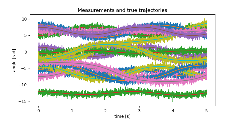
resultat shape (3000, 30)

Adapt the eoms for opty.

steep = 50.0
T = me.dynamicsymbols('T')


def step_diff(x, a, steep):
    """A differentiable approximation of the Heaviside function."""
    return 0.5 * (1.0 + sm.tanh(steep * (x - a)))

Replace the nondifferentiable Heaviside function with a differentiable approximation. Add the eom, suitable to make T(t) mimick the time t.

T = sm.Function('T')(t)

torques = []
for i in range(no_test):
    torque = F * T * sm.sin(omega*(T - delta)) * step_diff(T, delta,
                                                           steep)
    torques.append((A[i], torque * A[i].z))

KM = me.KanesMethod(N, q_ind=q, u_ind=u, kd_eqs=kd)
fr, frstar = KM.kanes_equations(bodies, forces + torques)
eom = kd.col_join(fr + frstar)
eom = eom.col_join(sm.Matrix([T.diff(t) - 1.0]))
MathJaxRepr(eom)

$$\left[\begin{matrix}- u_{0} + \dot{q}_{0}\\- u_{1} + \dot{q}_{1}\\- u_{2} + \dot{q}_{2}\\- u_{3} + \dot{q}_{3}\\- u_{4} + \dot{q}_{4}\\- u_{5} + \dot{q}_{5}\\- u_{6} + \dot{q}_{6}\\- u_{7} + \dot{q}_{7}\\- u_{8} + \dot{q}_{8}\\- u_{9} + \dot{q}_{9}\\- u_{10} + \dot{q}_{10}\\- u_{11} + \dot{q}_{11}\\- u_{12} + \dot{q}_{12}\\- u_{13} + \dot{q}_{13}\\- u_{14} + \dot{q}_{14}\\F \left(0.5 - 0.5 \tanh{\left(50.0 \delta - 50.0 T \right)}\right) T \sin{\left(\omega \left(- \delta + T\right) \right)} - g l m \sin{\left(q_{0} \right)} - \left(iZZ + l^{2} m\right) \dot{u}_{0}\\F \left(0.5 - 0.5 \tanh{\left(50.0 \delta - 50.0 T \right)}\right) T \sin{\left(\omega \left(- \delta + T\right) \right)} - g l m \sin{\left(q_{1} \right)} - \left(iZZ + l^{2} m\right) \dot{u}_{1}\\F \left(0.5 - 0.5 \tanh{\left(50.0 \delta - 50.0 T \right)}\right) T \sin{\left(\omega \left(- \delta + T\right) \right)} - g l m \sin{\left(q_{2} \right)} - \left(iZZ + l^{2} m\right) \dot{u}_{2}\\F \left(0.5 - 0.5 \tanh{\left(50.0 \delta - 50.0 T \right)}\right) T \sin{\left(\omega \left(- \delta + T\right) \right)} - g l m \sin{\left(q_{3} \right)} - \left(iZZ + l^{2} m\right) \dot{u}_{3}\\F \left(0.5 - 0.5 \tanh{\left(50.0 \delta - 50.0 T \right)}\right) T \sin{\left(\omega \left(- \delta + T\right) \right)} - g l m \sin{\left(q_{4} \right)} - \left(iZZ + l^{2} m\right) \dot{u}_{4}\\F \left(0.5 - 0.5 \tanh{\left(50.0 \delta - 50.0 T \right)}\right) T \sin{\left(\omega \left(- \delta + T\right) \right)} - g l m \sin{\left(q_{5} \right)} - \left(iZZ + l^{2} m\right) \dot{u}_{5}\\F \left(0.5 - 0.5 \tanh{\left(50.0 \delta - 50.0 T \right)}\right) T \sin{\left(\omega \left(- \delta + T\right) \right)} - g l m \sin{\left(q_{6} \right)} - \left(iZZ + l^{2} m\right) \dot{u}_{6}\\F \left(0.5 - 0.5 \tanh{\left(50.0 \delta - 50.0 T \right)}\right) T \sin{\left(\omega \left(- \delta + T\right) \right)} - g l m \sin{\left(q_{7} \right)} - \left(iZZ + l^{2} m\right) \dot{u}_{7}\\F \left(0.5 - 0.5 \tanh{\left(50.0 \delta - 50.0 T \right)}\right) T \sin{\left(\omega \left(- \delta + T\right) \right)} - g l m \sin{\left(q_{8} \right)} - \left(iZZ + l^{2} m\right) \dot{u}_{8}\\F \left(0.5 - 0.5 \tanh{\left(50.0 \delta - 50.0 T \right)}\right) T \sin{\left(\omega \left(- \delta + T\right) \right)} - g l m \sin{\left(q_{9} \right)} - \left(iZZ + l^{2} m\right) \dot{u}_{9}\\F \left(0.5 - 0.5 \tanh{\left(50.0 \delta - 50.0 T \right)}\right) T \sin{\left(\omega \left(- \delta + T\right) \right)} - g l m \sin{\left(q_{10} \right)} - \left(iZZ + l^{2} m\right) \dot{u}_{10}\\F \left(0.5 - 0.5 \tanh{\left(50.0 \delta - 50.0 T \right)}\right) T \sin{\left(\omega \left(- \delta + T\right) \right)} - g l m \sin{\left(q_{11} \right)} - \left(iZZ + l^{2} m\right) \dot{u}_{11}\\F \left(0.5 - 0.5 \tanh{\left(50.0 \delta - 50.0 T \right)}\right) T \sin{\left(\omega \left(- \delta + T\right) \right)} - g l m \sin{\left(q_{12} \right)} - \left(iZZ + l^{2} m\right) \dot{u}_{12}\\F \left(0.5 - 0.5 \tanh{\left(50.0 \delta - 50.0 T \right)}\right) T \sin{\left(\omega \left(- \delta + T\right) \right)} - g l m \sin{\left(q_{13} \right)} - \left(iZZ + l^{2} m\right) \dot{u}_{13}\\F \left(0.5 - 0.5 \tanh{\left(50.0 \delta - 50.0 T \right)}\right) T \sin{\left(\omega \left(- \delta + T\right) \right)} - g l m \sin{\left(q_{14} \right)} - \left(iZZ + l^{2} m\right) \dot{u}_{14}\\\dot{T} - 1.0\end{matrix}\right]$$

Set Up the Estimation Problem for opty

state_symbols = q + u + [T]

num_nodes = schritte
t0, tf = 0.0, interval
interval_value = (tf - t0) / (num_nodes - 1)

par_map = {}
par_map[m] = m1
par_map[g] = g1
par_map[l] = l1
par_map[iZZ] = iZZ1

If some measurement is more reliable than others its relative weight may be increased by setting the corresponding weight to a value larger than 1.0.

w = [1.0 for _ in range(no_test)]


def obj(free):
    summe = 0.0
    for i in range(no_test):
        summe += w[i] * interval_value * np.sum((measurement[:, i] -
                                                 free[i * num_nodes: (i + 1) *
                                                      num_nodes])**2)
    return summe


def obj_grad(free):
    grad = np.zeros_like(free)
    for i in range(no_test):
        grad[i * num_nodes: (i + 1) * num_nodes] = (-2 * w[i] *
                                                    interval_value *
                                                    (measurement[:, i] -
                                                     free[i * num_nodes:
                                                         (i + 1) * num_nodes]))
    return grad


instance_constraints = (
    T.func(t0) - t0,
)

Give rough bounds for the parameters to be erstimated. This speeds up the convergence.

bounds = {
    delta: (0.1, 2.0),
    omega: (1.0, 3.0),
    F: (0.1, 0.5),
}

prob = Problem(
    obj,
    obj_grad,
    eom,
    state_symbols,
    num_nodes,
    interval_value,
    known_parameter_map=par_map,
    instance_constraints=instance_constraints,
    bounds=bounds,
    time_symbol=t,
)

print('Sequence of unknown parameters in solution, to be estimated:',
      prob.collocator.unknown_parameters, '\n')

Sequence of unknown parameters in solution, to be estimated: (F, delta, omega)

As the measurements for the angles are known, it makes sense to use them as initial guess for the angles.

initial_guess = np.hstack((
    measurement.T.flatten(),  # initial guess for q
    np.zeros(no_test * num_nodes),  # initial guess for u
    np.linspace(t0, tf, num_nodes),  # initial guess for T
    [0.1, 1.0, 0.2],  # initial guess for F, omega, delta
))

Solve the problem.

solution, info = prob.solve(initial_guess)
print(info['status_msg'])

b'Algorithm terminated successfully at a locally optimal point, satisfying the convergence tolerances (can be specified by options).'

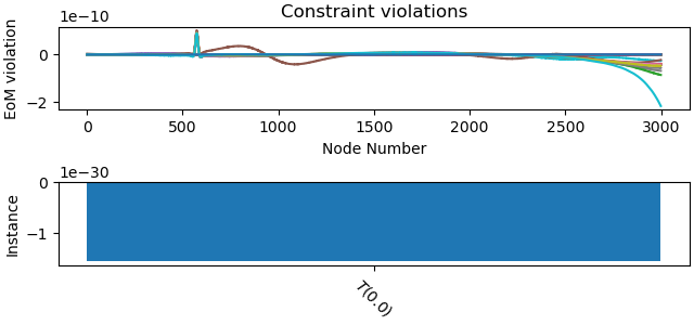
Plot the constraint violations.

_ = prob.plot_constraint_violations(solution)

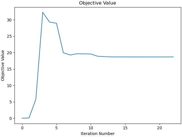
Plot the objective value as a function the the iterations.

_ = prob.plot_objective_value()

Print the results.

print((f'estimated \u03B4 = {solution[-2]:.3f}, given value = {delta1}, '
       f'hence error = {(solution[-2] - delta1)/delta1*100:.3f} %'))
print((f'estimated \u03C9 = {solution[-1]:.3f}, given value = {omega1},'
       f' hence error = {(solution[-1] - omega1)/omega1*100:.3f} %'))
print((f'estimated F = {solution[-3]:.3f}, given value = {F1},'
       f' hence error = {(solution[-3] - F1)/F1*100:.3f} %'))

estimated δ = 0.956, given value = 1.0, hence error = -4.367 %
estimated ω = 1.980, given value = 2.0, hence error = -0.991 %
estimated F = 0.243, given value = 0.25, hence error = -2.947 %

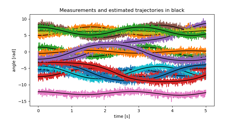
sphinx_gallery_thumbnail_number = 4

fig, ax = plt.subplots(figsize=(8, 4))
for i in range(no_test):
    ax.plot(times, measurement[:, i])
#    ax.plot(times, resultat[:, i], label=f'q{i+1}')
    ax.plot(times, solution[i*schritte:(i + 1)*schritte], color='black')
ax.set_xlabel('time [s]')
ax.set_ylabel('angle [rad]')
_ = ax.set_title('Measurements and estimated trajectories in black')