Nonconvex Delay (betts_10_90)

This is example 10.90 from John T. Betts, Practical Methods for Optimal Control Using NonlinearProgramming, 3rd edition, Chapter 10: Test Problems.

As reference, Betts gives: H. Mauer, Theory and applications of optimal control problems with control and state delays, Proceedings of the 53rd Australian Mathematical Confewrence, Adelaide, 2009.

This simulation shows the use of instance constrains of the form: \(x_i(t_0) = x_j(t_f)\).

States

• \(x_1,....., x_N\) : state variables

Controls

• \(u_1,....., u_N\) : control variables

import numpy as np
import sympy as sm
import sympy.physics.mechanics as me
from opty import Problem
from opty.utils import create_objective_function, MathJaxRepr

Equations of Motion

t = me.dynamicsymbols._t

N = 20
tf = 0.1
sigma = 5

x = me.dynamicsymbols(f'x:{N}')
u = me.dynamicsymbols(f'u:{N}')

eom = sm.Matrix([
    *[-x[i].diff(t) + 1**2 - u[i] for i in range(sigma)],
    *[-x[i].diff(t) + x[i-sigma]**2 - u[i] for i in range(sigma, N)],
])

MathJaxRepr(eom)

$$\left[\begin{matrix}- u_{0} - \dot{x}_{0} + 1\\- u_{1} - \dot{x}_{1} + 1\\- u_{2} - \dot{x}_{2} + 1\\- u_{3} - \dot{x}_{3} + 1\\- u_{4} - \dot{x}_{4} + 1\\- u_{5} + x_{0}^{2} - \dot{x}_{5}\\- u_{6} + x_{1}^{2} - \dot{x}_{6}\\- u_{7} + x_{2}^{2} - \dot{x}_{7}\\- u_{8} + x_{3}^{2} - \dot{x}_{8}\\- u_{9} + x_{4}^{2} - \dot{x}_{9}\\- u_{10} + x_{5}^{2} - \dot{x}_{10}\\- u_{11} + x_{6}^{2} - \dot{x}_{11}\\- u_{12} + x_{7}^{2} - \dot{x}_{12}\\- u_{13} + x_{8}^{2} - \dot{x}_{13}\\- u_{14} + x_{9}^{2} - \dot{x}_{14}\\- u_{15} + x_{10}^{2} - \dot{x}_{15}\\- u_{16} + x_{11}^{2} - \dot{x}_{16}\\- u_{17} + x_{12}^{2} - \dot{x}_{17}\\- u_{18} + x_{13}^{2} - \dot{x}_{18}\\- u_{19} + x_{14}^{2} - \dot{x}_{19}\end{matrix}\right]$$

Define and Solve the Optimization Problem

num_nodes = 501
t0 = 0.0
interval_value = (tf - t0) / (num_nodes - 1)

state_symbols = x
unkonwn_input_trajectories = u

Specify the objective function and form the gradient.

objective = sm.Integral(sum([x[i]**2 + u[i]**2 for i in range(N)]), t)

obj, obj_grad = create_objective_function(
    objective,
    state_symbols,
    unkonwn_input_trajectories,
    tuple(),
    num_nodes,
    interval_value
)

Instance Constraints and Bounds.

instance_constraints = (
    x[0].func(t0) - 1.0,
    *[x[i].func(t0) - x[i-1].func(tf) for i in range(1, N)],
)

limit_value = np.inf
bounds = {
   x[i]: (0.7, limit_value) for i in range(0, N)
}

Set Up the Control Problem and Solve it

prob = Problem(
    obj,
    obj_grad,
    eom,
    state_symbols,
    num_nodes,
    interval_value,
    instance_constraints=instance_constraints,
    bounds=bounds,
    time_symbol=t,
)

Rough initial guess.

initial_guess = np.ones(prob.num_free) * 0.1

Find the optimal solution.

solution, info = prob.solve(initial_guess)
print(info['status_msg'])
Jstr = 2.79685770
print(f"Objective value achieved: {info['obj_val']:.4f}, as per the book ",
      f"it is {Jstr:.4f}, so the error is: ",
      f"{(info['obj_val'] - Jstr) / Jstr * 100:.4f} % ")
print('\n')

b'Algorithm terminated successfully at a locally optimal point, satisfying the convergence tolerances (can be specified by options).'
Objective value achieved: 2.7967, as per the book  it is 2.7969, so the error is:  -0.0040 %

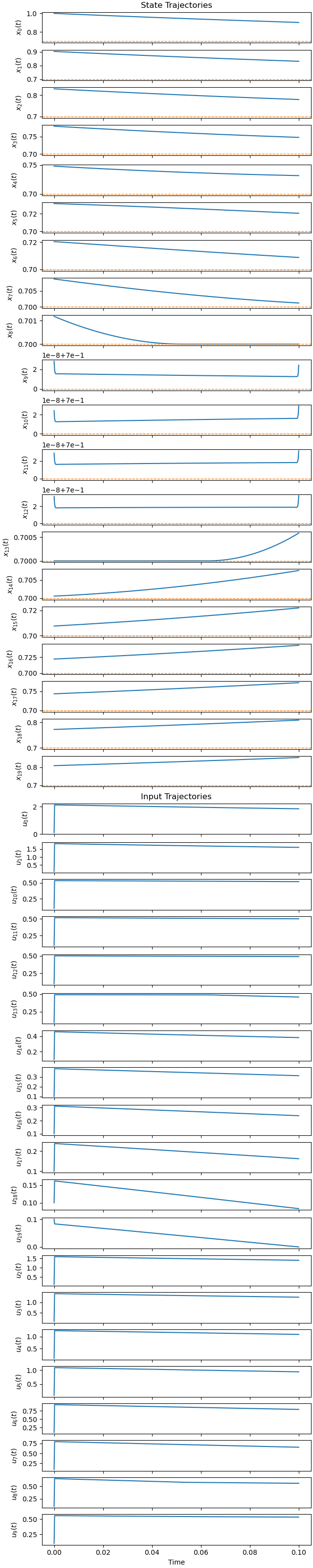
Plot the optimal state and input trajectories.

_ = prob.plot_trajectories(solution, show_bounds=True)

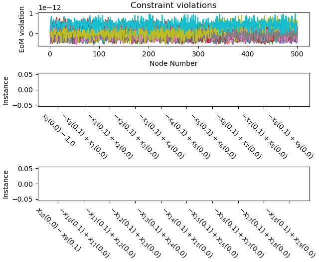
Plot the constraint violations.

_ = prob.plot_constraint_violations(solution)

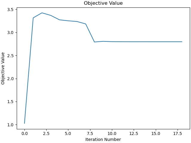
Plot the objective function.

_ = prob.plot_objective_value()

Are the inequality constraints strictly satisfied?

min_x = np.min(solution[0: N*num_nodes-1])
if min_x >= 0.7:
    print(f"Minimal value of the x\u1D62 is: {min_x:.12f} >= 0.7",
          "hence satisfied")
else:
    print(f"Minimal value of the x\u1D62 is: {min_x:.12f} < 0.7",
          "hence not satisfied")

Minimal value of the xᵢ is: 0.700000012530 >= 0.7 hence satisfied