Note
Go to the end to download the full example code.
Rotating T-handle
Objective
Show how to simulate the gyroscopic effects on a simple body in a region without gravity.
Description
This simulates a T - handle rotating where there is no gravity. The T-handle consists of two cylinders rigidly attached to each other at right angles.
The main rotation is around the A1.x axis, the other two rotations are the disturbances.They are around the A1.y and A1.z axis, and they are \(\dfrac{1}{100}\)-th in magnitude compared to the main rotation. A1 is the body fixed frame of one of the cylinders forming the T-handle.
The idea is based on this video: https://moorepants.github.io/learn-multibody-dynamics/angular.html
Notes
The T - handle is composed of two rods rigidly attached to each other, by aligning the A2 frame rigidly with the A1 frame. This way no need to think about what the moments of inertia for a T - handle would look like, sympy mechanics will take care.
The animation may be made to look nicer by increasing
zeitpunktebelow.
States
\(q_1, q_2, q_3\) are the angles of the T-handle
\(x, y, z\) are the coordinates of the center of mass of one of the cylinders forming the T-handle
\(u_1, u_2, u_3\) are the angular velocities
\(u_x, u_y, u_z\) are the velocities of the center of mass of one of the cylinders forming the T-handle
Parameters
\(l_1, l_2\) are the lengths of the cylinders
\(r_1, r_2\) are the radii of the cylinders
\(m_1, m_2\) are the masses of the cylinders
import sympy as sm
import sympy.physics.mechanics as me
import numpy as np
from scipy.integrate import solve_ivp
import matplotlib.pyplot as plt
from matplotlib.animation import FuncAnimation
import matplotlib as mp
mp.rcParams['animation.embed_limit'] = 2**128
Kane’s Equations of Motion
N, A1, A2 = sm.symbols('N A1 A2', cls=me.ReferenceFrame)
O, Dmc1, Dmc2, P1, P2, P3 = sm.symbols('O Dmc1 Dmc2 P1 P2 P3', cls=me.Point)
O.set_vel(N, 0)
t = me.dynamicsymbols._t
q1, q2, q3 = me.dynamicsymbols('q1 q2 q3')
u1, u2, u3 = me.dynamicsymbols('u1 u2 u3')
x, y, z = me.dynamicsymbols('x y z')
ux, uy, uz = me.dynamicsymbols('ux uy uz')
l1, l2, r1, r2, m1, m2, = sm.symbols('l1 l2 r1 r2 m1 m2')
# A1 is the body fixed frame of the first cylinder
A1.orient_body_fixed(N, (q1, q2, q3), '123')
# needed for the kinematic differential equations
rot = A1.ang_vel_in(N)
A1.set_ang_vel(N, u1*A1.x + u2*A1.y + u3*A1.z)
# needed for the kinematic differential equations
rot1 = A1.ang_vel_in(N)
# A1.x perpenducular to A2.x, A1.z parallel to A2.x.
A2.orient_axis(A1, sm.pi/2, A1.z)
# Dmc1 is the center of mass of the first cylinder
Dmc1.set_pos(O, x*N.x + y*N.y + z*N.z)
Dmc1.set_vel(N, ux*N.x + uy*N.y + uz*N.z)
# P1 is the point where the first cylinder is attached to the t handle
P1.set_pos(Dmc1, -l1/2*A1.x)
P1.v2pt_theory(Dmc1, N, A1)
# Dmc2 is the center of mass of the second cylinder
Dmc2.set_pos(Dmc1, l1/2*A1.x)
Dmc2.v2pt_theory(Dmc1, N, A1)
# P2 is the 'far left point' of the second cylinder
P2.set_pos(Dmc2, -l2/2*A2.x)
P2.v2pt_theory(Dmc2, N, A2)
# P3 is the 'far right point' of the second cylinder
P3.set_pos(Dmc2, l2/2*A2.x)
P3.v2pt_theory(Dmc2, N, A2)
# moments of inertia of the cylinders forming the t handle.
iXX1 = 0.5 * m1 * r1**2
iYY1 = 0.25*m1*r1**2 + 1/12*m1*l1**2
iZZ1 = iYY1
iXX2 = 0.5 * m2 * r2**2
iYY2 = 0.25*m2*r2**2 + 1/12*m2*l2**2
iZZ2 = iYY2
I1 = me.inertia(A1, iXX1, iYY1, iZZ1)
I2 = me.inertia(A2, iXX2, iYY2, iZZ2)
body1 = me.RigidBody('body1', Dmc1, A1, m1, (I1, Dmc1))
body2 = me.RigidBody('body2', Dmc2, A2, m2, (I2, Dmc2))
BODY = [body1, body2]
kd = [ux - x.diff(t), uy - y.diff(t), uz - z.diff(t)] + [me.dot(rot - rot1, uv)
for uv in N]
q_ind = [q1, q2, q3] + [x, y, z]
u_ind = [u1, u2, u3] + [ux, uy, uz]
KM = me.KanesMethod(N, q_ind=q_ind, u_ind=u_ind, kd_eqs=kd)
fr, frstar = KM.kanes_equations(BODY)
MM = KM.mass_matrix_full
force = KM.forcing_full
print('MM Ds', me.find_dynamicsymbols(MM))
print('MM FS', MM.free_symbols)
print((f'MM contains {sm.count_ops(MM)} operations, '
f'{sm.count_ops(sm.cse(MM))} after cse \n'))
print('forces Ds', me.find_dynamicsymbols(force))
print('forces FS', force.free_symbols)
print((f'forces contains {sm.count_ops(force)} operations, '
f'{sm.count_ops(sm.cse(force))} after cse \n'))
MM Ds {q2(t), q1(t), q3(t)}
MM FS {t, r2, l1, r1, l2, m2, m1}
MM contains 180 operations, 51 after cse
forces Ds {uy(t), q1(t), u1(t), ux(t), q3(t), u3(t), uz(t), q2(t), u2(t)}
forces FS {t, r2, l1, r1, l2, m2, m1}
forces contains 5310 operations, 215 after cse
Define a few functions needed for plotting and lambdify them.
P1_ort = [P1.pos_from(O).dot(N.x), P1.pos_from(O).dot(N.y),
P1.pos_from(O).dot(N.z)]
P2_ort = [P2.pos_from(O).dot(N.x), P2.pos_from(O).dot(N.y),
P2.pos_from(O).dot(N.z)]
P3_ort = [P3.pos_from(O).dot(N.x), P3.pos_from(O).dot(N.y),
P3.pos_from(O).dot(N.z)]
Dmc1_ort = [Dmc1.pos_from(O).dot(N.x), Dmc1.pos_from(O).dot(N.y),
Dmc1.pos_from(O).dot(N.z)]
Dmc2_ort = [Dmc2.pos_from(O).dot(N.x), Dmc2.pos_from(O).dot(N.y),
Dmc2.pos_from(O).dot(N.z)]
kin_energie = sum([body.kinetic_energy(N) for body in BODY])
qL = [q1, q2, q3, x, y, z] + [u1, u2, u3, ux, uy, uz]
pL = [l1, l2, r1, r2, m1, m2]
MM_lam = sm.lambdify(qL + pL, MM, cse=True)
force_lam = sm.lambdify(qL + pL, force, cse=True)
kin_energie_lam = sm.lambdify(qL + pL, kin_energie, cse=True)
p1_ort_lam = sm.lambdify(qL + pL, P1_ort, cse=True)
p2_ort_lam = sm.lambdify(qL + pL, P2_ort, cse=True)
p3_ort_lam = sm.lambdify(qL + pL, P3_ort, cse=True)
Dmc1_ort_lam = sm.lambdify(qL + pL, Dmc1_ort, cse=True)
Dmc2_ort_lam = sm.lambdify(qL + pL, Dmc2_ort, cse=True)
Numerical integration
The disturbances are the rotations around the A1.y, A1,z axes. Main rotation is around the A1.x axis.
x1, y1, z1 = 0, 0, 0 # location of Dmc1
ux1, uy1, uz1 = 0, 0, 0 # velocity of Dmc1
q11, q21, q31 = 0, 0, 0 # orientation of A1, that is of the t handle
# lengths of the cylinders composing the t handle, radius of the cylinders,
# mass of the cylinders
l11, l21, r11, r21, m11, m21 = 1, 2, 0.1, 0.1, 2, 1
u11 = 10 # angular velocity of A1.x
u21 = 1.e-1 # angular velocity of A1.y, the disturbance
u31 = 1.e-1 # angular velocity of A1.z, the disturbance
intervall = 10 # time of integration
schritte = 200 # number of steps per second duration-
y0 = [q11, q21, q31, x1, y1, z1, u11, u21, u31, ux1, uy1, uz1]
pL_vals = [l11, l21, r11, r21, m11, m21]
def gradient(t, y, args):
sol = np.linalg.solve(MM_lam(*y, *args), force_lam(*y, *args))
return np.array(sol).T[0]
times = np.linspace(0., intervall, int(schritte*intervall))
t_span = (0., intervall)
resultat1 = solve_ivp(gradient, t_span, y0, t_eval=times, args=(pL_vals,),
atol=1.e-12, rtol=1.e-12)
resultat = resultat1.y.T
print('Shape of result: ', resultat.shape)
print(resultat1.message)
print(f'solve_ivp made {resultat1.nfev:,} function calls')
Shape of result: (2000, 12)
The solver successfully reached the end of the integration interval.
solve_ivp made 14,978 function calls
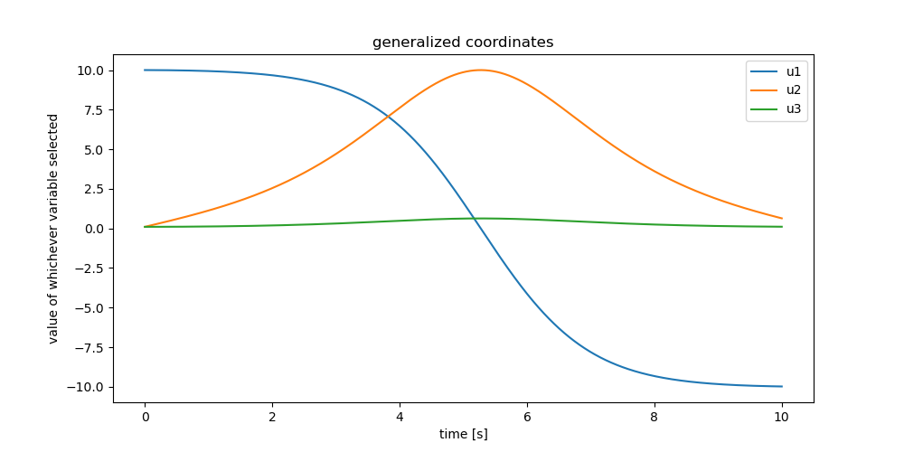
Plot whichever generalized coordinates you care to see.
fig, ax = plt.subplots(1, 1, figsize=(10, 5))
bezeichnung = ['q1', 'q2', 'q3', 'x', 'y', 'z', 'u1', 'u2',
'u3', 'ux', 'uy', 'uz']
for i in (6, 7, 8):
ax.plot(times, resultat[:, i], label=bezeichnung[i])
ax.set_xlabel('time [s]')
ax.set_ylabel('value of whichever variable selected')
ax.set_title('generalized coordinates')
_ = ax.legend()
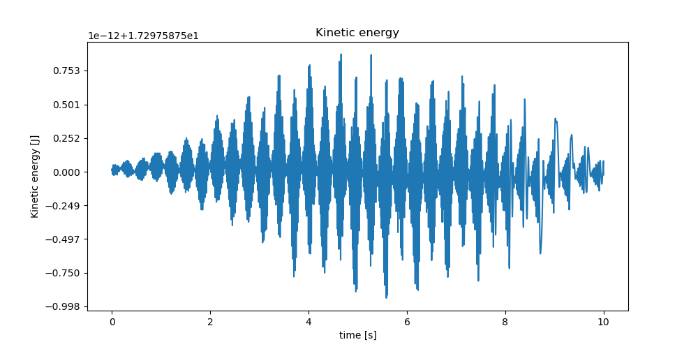
Energies of the system. The energy seems constant up to numerical errors.
coords = np.empty(resultat.shape[0])
for i in range(resultat.shape[0]):
coords[i] = kin_energie_lam(*resultat[i], *pL_vals)
fig, ax3 = plt.subplots(1, 1, figsize=(10, 5))
ax3.plot(times, coords)
ax3.set_title('Kinetic energy')
ax3.set_xlabel('time [s]')
_ = ax3.set_ylabel('Kinetic energy [J]')
Animate the T - handle
zeitpunkte = 100
times2 = []
resultat2 = []
index2 = []
reduction = max(1, int(len(times)/zeitpunkte))
for i in range(len(times)):
if i % reduction == 0:
times2.append(times[i])
resultat2.append(resultat[i])
resultat2 = np.array(resultat2)
schritte2 = len(times2)
P1_loc = np.empty((schritte2, 3))
P2_loc = np.empty((schritte2, 3))
P3_loc = np.empty((schritte2, 3))
Dmc2_loc = np.empty((schritte2, 3))
for i in range(schritte2):
P1_loc[i] = p1_ort_lam(*resultat2[i], *pL_vals)
P2_loc[i] = p2_ort_lam(*resultat2[i], *pL_vals)
P3_loc[i] = p3_ort_lam(*resultat2[i], *pL_vals)
Dmc2_loc[i] = Dmc2_ort_lam(*resultat2[i], *pL_vals)
xmin = min(np.min(np.abs(P1_loc)), np.min(np.abs(P2_loc)),
np.min(np.abs(P3_loc)), np.min(np.abs(Dmc2_loc)))
xmax = max(np.max(np.abs(P1_loc)), np.max(np.abs(P2_loc)),
np.max(np.abs(P3_loc)), np.max(np.abs(Dmc2_loc)))
fig = plt.figure(figsize=(8, 8))
ax = fig.add_subplot(111, projection='3d')
ax.set_aspect('equal')
ax.set_xlabel('X direction in N', fontsize=12)
ax.set_ylabel('Y direction in N', fontsize=12)
ax.set_zlabel('Z direction in N', fontsize=12)
xmin = xmin - 1.
xmax = xmax + 1.
ax.set_xlim(xmin, xmax)
ax.set_ylim(xmin, xmax)
ax.set_zlim(xmin, xmax)
# Inmitiate the lines
line1, = ax.plot([], [], [], 'r', lw=2)
line2, = ax.plot([], [], [], 'blue', lw=2)
# Function to update the plot in the animation
def update(frame):
message = (f'running time {times2[frame]:.2f}')
ax.set_title(message, fontsize=14)
line1.set_data([P1_loc[frame, 0], Dmc2_loc[frame, 0]],
[P1_loc[frame, 1], Dmc2_loc[frame, 1]])
line1.set_3d_properties([P1_loc[frame, 2], Dmc2_loc[frame, 2]])
line2.set_data([P2_loc[frame, 0], P3_loc[frame, 0]],
[P2_loc[frame, 1], P3_loc[frame, 1]])
line2.set_3d_properties([P2_loc[frame, 2], P3_loc[frame, 2]])
return line1, line2
ax.view_init(elev=30, azim=30, roll=0.)
# Create the animation
ani = FuncAnimation(fig, update, frames=schritte2,
interval=1000*np.max(times2) / schritte2)
plt.show()