Note
Go to the end to download the full example code.
Nonminimal Double Pendulum using Lagrange’s Method
Objectives
Formulate the equations of motion for a nonminimal double pendulum using
sympy.physics.mechanics, Lagrange method.Implement the
stabilized (Hiller and Anatharaman) index 1 formulationfor solving the resulting differential-algebraic equations.Show how to use
solve_daeto integrate the DAEs of motion.
Description
A double pendulum consisting of two bars of equal length \(l\) and mass \(m\) is attached to the origin. There may be friction in the joints and a spring connecting the two pendulums ‘wants’ to keep them aligned.The positions of the end points of the pendulums are described by the coordinates \(x_1, y_1, x_2, y_2\).
Of course the simplest way to model a double pendulum is to use the minimal coordinates (angles), but here we use the nonminimal coordinates (cartesian coordinates of the pendulum masses), giving two holonomic constraints \(x_1^2 + y_1^2 - l^2 = 0, \quad x_2^2 + y_2^2 - l^2 = 0\). This shows how to proceed in such a case.
Notes
If \(k_{\textrm{spring}} > 0\) it must be large enough to kee the pendulums from rotating into each other. Otherwise the model is no longer valid.
States
\(x_1, y_1, x_2, y_2\) : Coordinates of the two pendulums. Note: x2 and y2 are relative to the first pendulum.
\(\lambda_1, \lambda_2\) : Lagrange multipliers corresponding to the constraints.
\(\dot{\lambda}_1, \dot{\lambda}_2\) : Time derivatives of the Lagrange multipliers. In the Hiller and Anatharaman index 1 formulation, these time derivatives are used to stabilize the integration.
\(\nu_1, \nu_2\) : Stabilizing multipliers for the index 1 formulation.
\(\dot{\nu}_1, \dot{\nu}_2\) : Time derivatives of the stabilizing multipliers. Only these time derivatives are of significance.
Parameters
\(m\) : Mass of each pendulum.
\(l\) : Length of each pendulum.
\(g\) : Gravitational acceleration.
\(\textrm{reibung}\) : Friction coefficient in the joints.
\(k_{\textrm{spring}}\) : Spring constant of the spring connecting the two pendulums.
import sympy as sm
import sympy.physics.mechanics as me
import numpy as np
from solve_dae.integrate import solve_dae, consistent_initial_conditions
import matplotlib.pyplot as plt

from scipy.interpolate import interp1d
from matplotlib.animation import FuncAnimation
Set up the Equations of Motion using Lagrange Method
N, A1, A2 = sm.symbols('N A1, A2', cls=me.ReferenceFrame)
O, P1, P2 = sm.symbols('O P1 P2', cls=me.Point)
x1, y1, x2, y2 = me.dynamicsymbols('x1 y1 x2 y2')
t = me.dynamicsymbols._t
O.set_vel(N, 0)
P1.set_pos(O, x1 * N.x + y1 * N.y)
P1.set_vel(N, P1.pos_from(O).diff(t, N))

P2.set_pos(P1, x2 * N.x + y2 * N.y)
P2.set_vel(N, P2.pos_from(O).diff(t, N))

A1.orient_axis(N, sm.atan2(y1, x1), N.z)
A2.orient_axis(N, sm.atan2(y2, x2), N.z)

m, g, l, reibung, k_spring = sm.symbols('m g l reibung k_spring')

Inert1 = me.inertia(A1, 0, 0, 1/3 * m * l**2)
Pa1 = me.RigidBody('Pa1', P1, A1, m, (Inert1, P1))
Inert2 = me.inertia(A2, 0, 0, 1/3 * m * l**2)
Pa2 = me.RigidBody('Pa2', P2, A2, m, (Inert2, P2))
This is to get the torques on A1, A2 to act in the right direction.
hilfs = P1.pos_from(O).cross(P2.pos_from(P1))
hilfs_z = hilfs.dot(N.z)
hilfs_R = sm.Piecewise((1, hilfs_z > 0), (-1, True))
sinwinkel = hilfs.magnitude() / l**2
winkel = sm.asin(sinwinkel)
Set up the forcelist.
FL = [(P1, -m * g * N.y - reibung * (x1.diff(t) * N.x + y1.diff(t) * N.y)),
      (P2, -m * g * N.y - reibung * (x2.diff(t) * N.x + y2.diff(t) * N.y)),
      (A1, k_spring * hilfs_R * winkel * N.z),
      (A2, -k_spring * hilfs_R * winkel * N.z)
      ]
Lengths of the pendulums are constant.
config_constr = sm.Matrix([x1**2 + y1**2 - l**2, x2**2 + y2**2 - l**2])
Lagrangian function.
Here only the kinetic energy is given. The potential energies (here gravitation and spring energy) can either be given in the Lagrangian function or included in the force list - but NOT in both! Here the gravitational potential energy and the spring potential energy are included in the force list, not in the Lagrangian.
lag = me.Lagrangian(N, Pa1, Pa2)
Form the Lagrange object.
LM = me.LagrangesMethod(lag, [x1, y1, x2, y2], hol_coneqs=config_constr,
                        forcelist=FL, frame=N)
Equations of motion. They contain one Lagrange multiplier for each constraint, so here we have \(\lambda_1\) and \(\lambda_2\).
lag_eqs = LM.form_lagranges_equations()
Parameters.
m1 = 1.0
l1 = 2.0
g1 = 9.81
reibung1 = 0.0
k_spring1 = 17.5

pL = [m, l, g, reibung, k_spring]
pL_vals = [m1, l1, g1, reibung1, k_spring1]
pL_dict = {i: j for i, j in zip(pL, pL_vals)}
For solve_dae we need v and vp where \(vp = \dfrac{dv}{dt}\)
So we define the initial conditionsa in terms of v.
v01 = l1 / np.sqrt(2)  # corresponds to x1
v11 = l1 / np.sqrt(2)  # corresponds to y1
v21 = l1 / np.sqrt(2)   # corresponds to x2
v31 = l1 / np.sqrt(2)   # corresponds to y2
v41 = 1.0   # corresponds to x1.diff(t)
v51 = -1.0   # corresponds to y1.diff(t)
v61 = 1.0   # corresponds to x2.diff(t)
v71 = -1.0   # corresponds to y2.diff(t)
v81 = 0.0   # corresponds to lam1
v91 = 0.0   # corresponds to lam2
v101 = 0.0   # corresponds to nu1
v111 = 0.0   # corresponds to nu2
Set up for solve_dae
This formulation is known as Hiller and Anatharaman or stabilized index 1 formulation. (From Jonas Breuling, private communication)
\(g(q) \in \\R^2, q, u \in \\R^4\).
Set \(W^T(q) := \dfrac{\partial}{\partial{q}}g(q)\)
F = \(\begin{pmatrix} \dot{q} - u - \dfrac{\partial}{\partial{q}}g(t, q)^T \cdot \dot{\nu} \\ M(q) \cdot \dot{u} - h(q, u) - \dfrac{\partial}{\partial{q}}g^T(q) \cdot \dot{\lambda} \\ \dfrac{d}{dt} g(q) \\ g(q) \end{pmatrix} \in \\R^{12}\)
Below is needed to replace the variables used in setting up the DAE
system with the variables needed for solve_dae.
I may not have done this the most efficient way.
h1, h2 = me.dynamicsymbols('h1 h2')
nu1, nu2 = me.dynamicsymbols('nu1 nu2')
nu1dt, nu2dt = nu1.diff(t), nu2.diff(t)
lam1, lam2 = me.dynamicsymbols('lam1 lam2')
lam1dt, lam2dt = lam1.diff(t), lam2.diff(t)
I did not manage to replace lam_i with lam_i.diff(t) directly as required by Hiller Anathanraman. So I had to go the detour via h1, h2.
lag_eqs1 = me.msubs(lag_eqs, {lam1: h1, lam2: h2})
Create \(W = \left(\frac{\partial g}{\partial q}\right)^T\) as the Jacobian of the constraints with respect to the generalized coordinates.
W = config_constr.jacobian([x1, y1, x2, y2])
W = W.T
Time derivative of the constraint matrix.
speed_constr = config_constr.diff(t)
Variables needed for solve_dae.
v = me.dynamicsymbols('v:12')
vp = me.dynamicsymbols('vp:12')
First equation.
F0 = (sm.Matrix([vp[i] - v[i+4] for i in range(4)]) -
      W * sm.Matrix([nu1dt, nu2dt]))
Second equation.
F1 = lag_eqs1
Third equation.
F2 = speed_constr
Fourth equation.
F3 = config_constr
Replace original variables.
v_dict = {x1: v[0], y1: v[1], x2: v[2], y2: v[3],
          x1.diff(t): v[4], y1.diff(t): v[5], x2.diff(t): v[6],
          y2.diff(t): v[7],
          lam1: v[8], lam2: v[9], nu1: v[10], nu2: v[11]}
vp_dict = ({key.diff(t): vp[i] for i, key in enumerate(v_dict.keys())}
           | {h1: vp[8], h2: vp[9]})
It is important to replace in sequence, otherwise it may not work.
F0 = me.msubs(F0, v_dict)
F0 = me.msubs(F0, vp_dict)

F1 = me.msubs(F1, v_dict)
F1 = me.msubs(F1, vp_dict)

F2 = me.msubs(F2, v_dict)
F2 = me.msubs(F2, vp_dict)

F3 = me.msubs(F3, v_dict)
F3 = me.msubs(F3, vp_dict)
Combine all equations into a single matrix.
eom_dae = sm.Matrix([F0, F1, F2, F3])
Compile it.
eom_dae_lam = sm.lambdify(v + vp + pL, eom_dae, cse=True)
Define the energies: kinetic, potential, and spring.
kin_energy = Pa1.kinetic_energy(N) + Pa2.kinetic_energy(N)
pot_energy = m * g * (P1.pos_from(O).dot(N.y) + P2.pos_from(O).dot(N.y))
spring_energy = 1/2 * k_spring * winkel**2
kin_energy = me.msubs(kin_energy, v_dict)
kin_energy = me.msubs(kin_energy, vp_dict)
pot_energy = me.msubs(pot_energy, v_dict)
pot_energy = me.msubs(pot_energy, vp_dict)
spring_energy = me.msubs(spring_energy, v_dict)
spring_energy = me.msubs(spring_energy, vp_dict)
Compile them.
kin_lam = sm.lambdify(v + vp + pL, kin_energy, cse=True)
pot_lam = sm.lambdify(v + vp + pL, pot_energy, cse=True)
spring_lam = sm.lambdify(v + vp + pL, spring_energy, cse=True)
Integrate the Equations of Motion using the DAE Solver
def gradient_dae(t, v, vp):
    return eom_dae_lam(*v, *vp, *pL_vals).squeeze()


v0_start = [v01, v11, v21, v31, v41, v51, v61, v71, v81, v91, v101, v111]
vp0_start = [0.0] * len(v0_start)
Enforce consistent initial conditions.
v01_j, vp01_j, f0 = consistent_initial_conditions(gradient_dae, 0.0, v0_start,
                                                  vp0_start)
print('v01_j', v01_j)
print('vp01_j', vp01_j)
v01_j [ 1.41421356  1.41421356  1.41421356  1.41421356  1.         -1.
  1.         -1.          0.          0.          0.          0.        ]
vp01_j [ 2.          0.          2.          0.          0.         -7.74473684
  0.         -1.54894737 -0.45636299 -0.0912726   0.35355339  0.35355339]
The initial conditions must satisfy the equations of motion, so this norm should be close to zero.
print('norm(f0) = ', np.linalg.norm(f0))
norm(f0) = 3.225018736278932e-14
Integration starts. stages must be a positive and odd integer. Default is 3
stages = 5
Meaning of these parameters virtually identical to scipy’s solve_ivp.
rtol = 1e-3
atol = 1e-6
t0, tf = 0.0, 10.0
schritte = 500
times = np.linspace(t0, tf, schritte)
method_dae = 'Radau'
sol = solve_dae(gradient_dae,
                (t0, tf),
                v01_j,
                vp01_j,
                atol=atol,
                rtol=rtol,
                method=method_dae,
                t_eval=times,
                stages=stages,
                )

values = sol.y
derivatives = sol.yp

success = sol.success
status = sol.status
message = sol.message
print(f"success: {success}")
print(f"status: {status}")
print(f"message: {message}")
print(f"nfev: {sol.nfev}")
print(f"njev: {sol.njev}")
print(f"nlu: {sol.nlu}")
success: True
status: 0
message: The solver successfully reached the end of the integration interval.
nfev: 3946
njev: 108
nlu: 606
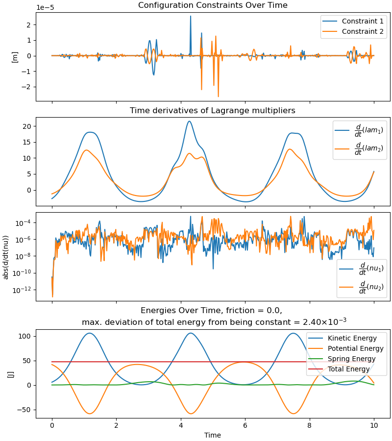
Check how well the holonomic constraints are kept.
Plot the Lagrange multipliers. Only their time derivatives have physical meaning.
Total energy should be constant iff friction = 0.
config_constr_lam = sm.lambdify([x1, y1, x2, y2] + pL, config_constr)
constr1_np = config_constr_lam(sol.y[0, :], sol.y[1, :], sol.y[2, :],
                               sol.y[3, :], *pL_vals)[0]
constr2_np = config_constr_lam(sol.y[0, :], sol.y[1, :], sol.y[2, :],
                               sol.y[3, :], *pL_vals)[1]

fig, ax = plt.subplots(4, 1, figsize=(8, 9), sharex=True, layout='constrained')
ax[0].plot(sol.t, constr1_np.T, label='Constraint 1')
ax[0].plot(sol.t, constr2_np.T, label='Constraint 2')
ax[-1].set_xlabel('Time')
ax[0].set_ylabel('[m]')
ax[0].set_title('Configuration Constraints Over Time')
ax[0].legend()

ax[1].plot(sol.t, sol.yp[8, :], label='$\dfrac{d}{dt}(lam_1)$')
ax[1].plot(sol.t, sol.yp[9, :], label='$\dfrac{d}{dt}(lam_2)$')
ax[1].legend()
ax[1].set_title('Time derivatives of Lagrange multipliers')
ax[2].plot(sol.t, np.abs(sol.yp[10, :]), label='$\dfrac{d}{dt}(nu_1)$')
ax[2].plot(sol.t, np.abs(sol.yp[11, :]), label='$\dfrac{d}{dt}(nu_2)$')
ax[2].set_ylabel('abs(d/dt(nu))')
ax[2].set_yscale('log')
ax[2].legend()

kin_np = kin_lam(*sol.y, *sol.yp, *pL_vals)
pot_np = pot_lam(*sol.y, *sol.yp, *pL_vals)
spring_np = spring_lam(*sol.y, *sol.yp, *pL_vals)
total_np = kin_np + pot_np + spring_np
max_total = np.max(total_np)
min_total = np.min(total_np)

delta = (max_total - min_total)
exponent = int(np.floor(np.log10(abs(delta))))
mantissa = delta / 10**exponent

ax[3].plot(sol.t, kin_np.T, label='Kinetic Energy')
ax[3].plot(sol.t, pot_np.T, label='Potential Energy')
ax[3].plot(sol.t, spring_np.T, label='Spring Energy')
ax[3].plot(sol.t, total_np.T, label='Total Energy')
ax[3].set_title(f'Energies Over Time, friction = {reibung1}, \n '
                'max. deviation of total energy from being'
                rf' constant = {mantissa:.2f}$\times10^{{{exponent}}}$')
ax[3].set_ylabel('[J]')
_ = ax[3].legend()
C:\Users\Peter\github_repos\pst-notebooks\gallery\plot_Lagrange_pendulum.py:359: SyntaxWarning: invalid escape sequence '\d'
  ax[1].plot(sol.t, sol.yp[8, :], label='$\dfrac{d}{dt}(lam_1)$')
C:\Users\Peter\github_repos\pst-notebooks\gallery\plot_Lagrange_pendulum.py:360: SyntaxWarning: invalid escape sequence '\d'
  ax[1].plot(sol.t, sol.yp[9, :], label='$\dfrac{d}{dt}(lam_2)$')
C:\Users\Peter\github_repos\pst-notebooks\gallery\plot_Lagrange_pendulum.py:363: SyntaxWarning: invalid escape sequence '\d'
  ax[2].plot(sol.t, np.abs(sol.yp[10, :]), label='$\dfrac{d}{dt}(nu_1)$')
C:\Users\Peter\github_repos\pst-notebooks\gallery\plot_Lagrange_pendulum.py:364: SyntaxWarning: invalid escape sequence '\d'
  ax[2].plot(sol.t, np.abs(sol.yp[11, :]), label='$\dfrac{d}{dt}(nu_2)$')
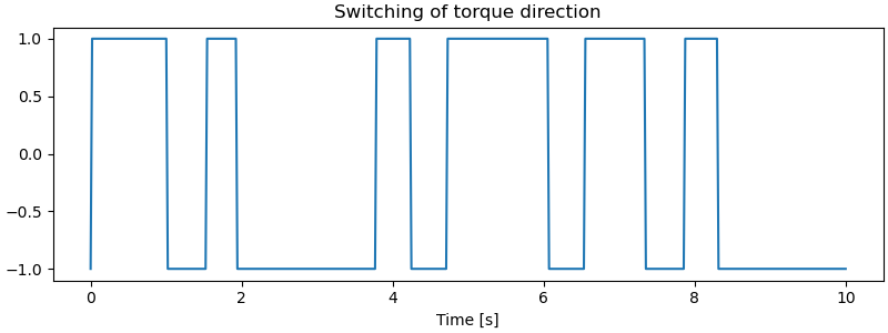
Direction of the torque.
winkel = me.msubs(hilfs_R, v_dict)
winkel_lam = sm.lambdify(v + pL, winkel)

fig, ax = plt.subplots(figsize=(8, 3), layout='constrained')
ax.plot(sol.t, winkel_lam(*sol.y, *pL_vals))
ax.set_xlabel('Time [s]')
_ = ax.set_title('Switching of torque direction')
Animation
fps = 15
qL = [x1, y1, x2, y2]
resultat = sol.y.T

t_arr = np.linspace(t0, tf, len(sol.t))
state_sol = interp1d(t_arr, resultat, kind='cubic', axis=0)

# Get the coordinates of the points in the inertial frame for plotting.
coords = P1.pos_from(O).to_matrix(N)
coords = coords.row_join(P2.pos_from(O).to_matrix(N))
coords_lam = sm.lambdify(qL + pL, coords, cse=True)


fig, ax = plt.subplots(figsize=(7, 7), layout='constrained')

min_x = -2*l1 - 0.25
max_x = 2*l1 + 0.25
min_y = -2*l1 - 0.25
max_y = 2*l1 + 0.25
ax.set_xlim(min_x, max_x)
ax.set_ylim(min_y, max_y)
ax.set_xlabel('x', fontsize=15)
ax.set_ylabel('y', fontsize=15)

ax.scatter(0.0, 0.0, s=75, color='blue', marker='v')
line1, = ax.plot([], [], color='blue', linewidth=1)
line2, = ax.plot([], [], color='blue', linewidth=1)
scatter1 = ax.scatter([], [], s=25, color='red', marker='o')
scatter2 = ax.scatter([], [], s=25, color='red', marker='o')


def update(frame):
    t = frame
    coords_vals = coords_lam(*state_sol(t)[0:4], *pL_vals)
    ax.set_title(f"Running time: {t:.2f} sec")

    line1.set_data([0, coords_vals[0, 0]], [0, coords_vals[1, 0]])
    line2.set_data([coords_vals[0, 0], coords_vals[0, 1]], [coords_vals[1, 0],
                                                            coords_vals[1, 1]])
    scatter1.set_offsets([coords_vals[0, 0], coords_vals[1, 0]])
    scatter2.set_offsets([coords_vals[0, 1], coords_vals[1, 1]])
    return line1, line2, scatter1, scatter2


ani = FuncAnimation(fig, update,
                    frames=np.concatenate((np.arange(0, tf, 1.0/fps),
                                           np.array([tf]))),
                    interval=1000/fps, blit=False)

plt.show()
Total running time of the script: (0 minutes 36.071 seconds)