Note
Go to the end to download the full example code.
Colliding Ellipses
Objectives
Show how to use Hunt-Crossley’s method to model collisions between ellipses and between ellipses and a circular wall.
Show how to use Kane’s method to get the equations of motion for the system. The forces are the main difficulty.
Show a somewhat nontrivial right hand side for
solve_ivpwhere the distances and speeds have to be calculated numerically for every step of the integration.
Description
n homogenious ellipses, named \(Dmc_0....Dmc_{n-1}\) with semi axes \(a, b\) and mass \(m_0\) are sliding frictionlessly on the horizontal X/Z plane.
Their space is limited by a circular wall of radius \(R_W\) with center at the origin. An observer, a particle of mass \(m_o\) may be attached anywhere within each ellipse.
To model the collisions, I use Hunt Crossley’s method
The reference is this article:
https://www.sciencedirect.com/science/article/pii/S0094114X23000782
This is with dissipation during the collision, the general force is given in (63) as
\(f_n = k_0 \cdot \rho + \chi \cdot \dot \rho\),
with \(k_0\) as below,
\(\rho\) the penetration,
and
\(\dot\rho\) the speed of the penetration.
Of course, \(\rho, \dot\rho\) must be the signed magnitudes of the respective vectors.
A more realistic force is given in (64) as:
\(f_n = k_0 \cdot \rho^n + \chi \cdot \rho^n\cdot \dot \rho\), as this avoids discontinuity at the moment of impact.
In the article it is stated, that \(n = \frac{3}{2}\) is a good choice, it is derived in Hertz’ approach.
Hunt and Crossley give this value for \(\chi\), see table 1:
\(\chi = \dfrac{3}{2} \cdot(1 - c_\tau) \cdot \dfrac{k_0}{\dot \rho^{(-)}}\)
where
\(c_\tau = \dfrac{v_1^{(+)} - v_2^{(+)}}{v_1^{(-)} - v_2^{(-)}}\),
where
\(v_i^{(-)}, v_i^{(+)}\) are the speeds of \(\textrm{body}_i\), before and after the collosion, see (45), \(\dot\rho^{(-)}\) is the speed right at the time the impact starts. \(c_\tau\) is an experimental factor, apparently around 0.8 for steel.
Using (64), this results in their expression for the force:
\(f_n = k_0 \cdot \rho^n \left[1 + \dfrac{3}{2} \cdot(1 - c_\tau) \cdot \dfrac{\dot\rho}{\dot\rho^{(-)}}\right]\)
with
\(k_0 = \frac{4}{3\cdot(\sigma_1 + \sigma_2)} \cdot \sqrt{\frac{R_1 \cdot R_2}{R_1 + R_2}}\),
where
\(\sigma_i = \frac{1 - \nu_i^2}{E_i}\)
with
\(\nu_i\) = Poisson’s ratio, \(E_i\) = Young’s modulus, \(R_1, R_2\) the radii of the colliding bodies, \(\rho\) the penetration depth. All is near equations (54) and (61) of this article.
As per the article, \(n = \frac{3}{2}\) is always to be used. (If I understood correctly, Hertz arrived at this exponent on theoretical grounds)
spring energy = \(k_0 \cdot \int_{0}^{\rho} k^{3/2}\,dk\) = \(k_0 \cdot\frac{2}{5} \cdot \rho^{5/2}\) I assume, the dissipated energy cannot be given in closed form, at least the article does not give one.
Notes
\(c_\tau = 1\) gives Hertz’s solution to the impact problem, also described in the article.
From the ellipse’s’ point of view, the wall is concave. I model this by taking \(R_2 = -R_W\). As \(max(a, b)| < |R_2|\) this will give no mathematical problems. I do not know, whether this approach is physically correct.
For more than two ellipses, integration runs a very long time, hours.
The animation can be made smoother by increasing the value of
zeitpunktein the animation part.
Variables / Parameters
\(n\) : number of ellipses
\(q_0...q_{n-1}\): generalized coordinates for the ellipses
\(u_0...u_{n-1}\): the angular speeds
\(x_i, z_i\): the coordinates, in the inertial frame \(N\), of the center of the i-th ellipse
\(N\): frame of inertia
\(P_0\): point fixed in \(N\)
\(A_i\): body fixed frame of the i-th ellipse
\(m_i\): mass of the i-th ellipse
\(Dmc_i\): center of the i-th ellipse
\(Po_i\): observer (particle) on i-th ellipse
\(\alpha_i, \beta_i\): distance of observer on i-th ellipse
\(a, b, R_W\): semi axes of the ellipses, radius of the wall
\(i_{YY_i}\): moment of inertia of the i-th ellipse
\(\text{reibung}\): coefficient of friction between ellipses / between ellipse and wall.
\(\nu_e, \nu_w\): Poison’s coefficients of the ellipses / of the wall
\(EY_e, EY_w\): dto for Young’s moduli
\(c_\tau\): the experimental constant needed for Hunt-Crossley
\(rhodt_{max}\): the collision speed between two ellipses, to be determined during integration, needed for Hunt_Crossley
\(rhodt_{wall}\): the collision speeds when $disc_i$ hits a wall
\(CPh_i\): contact point of \(\textrm{ellipse_i}\) with the wall
\(CPhs_i\): point on the ellipse which has had contact with the wall.
\(|{}^{CPh_i} r^{CPhs_i}|\) is the penetration depth.
\(CPhe_i\): potential contact points of \(\textrm{ellipse_i}\) with \(\textrm{ellipse_j}\). Penetration depth is \(|{}^{CPhe_i} r^{CPhe_j}|\)
\(l_{\textrm{list}}, le_{\textrm{list}}\): lists holding the penetration depth of \(\textrm{ellipse_i}\) with the wall / penetration depth of \(\textrm{ellipse_i}\) and \(\textrm{ellipse_j}\).
\(\textrm{epsilon}_{\textrm{list}}, \textrm{epsilone}_{\textrm{list}}\): lists holding the angles of the different contact points as discribed in the body fixed frames \(A_i\).
import sympy.physics.mechanics as me
import sympy as sm
from scipy.integrate import solve_ivp
from scipy.optimize import minimize, root
import numpy as np
from itertools import permutations
import matplotlib.pyplot as plt
from matplotlib import animation
from matplotlib import patches
import matplotlib as mp
mp.rcParams['animation.embed_limit'] = 2**126
This is needed to exit a loop, when a feasible initial location of the discs within the limitations of the wall was found.
class Rausspringen(Exception):
pass
Set up the geometry.
n = 2 # n > 1
if isinstance(n, int) is False or n < 2:
raise Exception('n must be an integer larger than 1')
q_list = me.dynamicsymbols(f'q:{n}')
u_list = me.dynamicsymbols(f'u:{n}')
x_list = me.dynamicsymbols(f'x:{n}')
z_list = me.dynamicsymbols(f'z:{n}')
ux_list = me.dynamicsymbols(f'ux:{n}')
uz_list = me.dynamicsymbols(f'uz:{n}')
CPh_list = list(sm.symbols(f'CPh:{n}', cls=me.Point))
CPhx_list = list(sm.symbols(f'CPhx:{n}'))
CPhz_list = list(sm.symbols(f'CPhz:{n}'))
CPhs_list = list(sm.symbols(f'CPhs:{n}', cls=me.Point))
CPhsx_list = list(sm.symbols(f'CPhsx:{n}'))
CPhsz_list = list(sm.symbols(f'CPhsz:{n}'))
A_list = sm.symbols(f'A:{n}', cls=me.ReferenceFrame)
Dmc_list = sm.symbols(f'Dmc:{n}', cls=me.Point)
Po_list = sm.symbols(f'Po:{n}', cls=me.Point)
alpha_list = list(sm.symbols(f'alpha:{n}'))
beta_list = list(sm.symbols(f'beta:{n}'))
epsilon_list = list(sm.symbols(f'epsilon:{n}'))
l_list = list(sm.symbols(f'l:{n}'))
rhodtmax = [sm.symbols(f'rhodtmax{i}{j}')
for i, j in permutations(range(n), r=2)]
le_list = [sm.symbols(f'le{i}{j}')
for i, j in permutations(range(n), r=2)]
epsilone_list = [sm.symbols(f'epsilone{i}{j}, epsilone{j}{i}')
for i, j in permutations(range(n), r=2)]
rhodtwall = list(sm.symbols(f'rhodtwall:{n}'))
richtung_list = [sm.symbols(f'richtungx{i}, richtungz{j}')
for i, j in permutations(range(n), r=2)]
t = me.dynamicsymbols._t
m0, mo, iYY, a, b, RW, nue = sm.symbols('m0, mo, iYY, a, b, RW, nue')
nuw, EYe, EYw, ctau, reibung = sm.symbols('nuw, EYe, EYw, ctau, reibung')
N = me.ReferenceFrame('N')
P0 = me.Point('P0')
P0.set_vel(N, 0)
Body1 = []
Body2 = []
for i in range(n):
A_list[i].orient_axis(N, q_list[i], N.y)
A_list[i].set_ang_vel(N, u_list[i] * N.y)
Dmc_list[i].set_pos(P0, x_list[i]*N.x + z_list[i]*N.z)
Dmc_list[i].set_vel(N, ux_list[i]*N.x + uz_list[i]*N.z)
Po_list[i].set_pos(Dmc_list[i], a * alpha_list[i] * A_list[i].x + b *
beta_list[i] * A_list[i].z)
Po_list[i].v2pt_theory(Dmc_list[i], N, A_list[i])
Ib = me.inertia(A_list[i], 0, iYY, 0)
body = me.RigidBody('body' + str(i), Dmc_list[i], A_list[i], m0,
(Ib, Dmc_list[i]))
teil = me.Particle('teil' + str(i), Po_list[i], mo)
Body1.append(body)
Body2.append(teil)
BODY = Body1 + Body2
Find the point where the ellipse hits the wall
If \(CP_h \in \textrm{circumference of the ellipse}\) is a potential collision point, then its ‘counterpart’ \(CP_{hs} \in \textrm{wall}\) must be on the line through \(P_0, CP_h\) where \(P_0\) is the center of the circular wall. Obviously \(|{}^{P_0} \bar r^{CP_{hs}}| = R_W\), the radius of the circular wall.
I try to find the pair \((CP_h , CP_{hs})\), which has the shortest distance from each other. This minimum is essentially [up to points \((q, m_x, m_z) \in \\R^3\) of Lebesque measure zero] unique- still minimize(..) does not always find it, see below. The \(\nabla\) - method does not work well here. I think, this is so because the distance does not depend continuously on \((q, m_x, m_z)\).
lang = sm.symbols('lang')
CPh = [sm.symbols('CPh' + str(i), cls=me.Point) for i in range(n)]
CPhs = [sm.symbols('CPhs' + str(i), cls=me.Point) for i in range(n)]
def CPhxe(epsilon):
return a * sm.cos(epsilon)
def CPhze(epsilon):
return b * sm.sin(epsilon)
CPh_list = []
CPhs_list = [] # just needed for the plot of the initial conditions
# define CPh
for i in range(n):
CPh[i].set_pos(Dmc_list[i], CPhxe(epsilon_list[i])*A_list[i].x +
CPhze(epsilon_list[i])*A_list[i].z)
nhat_hilfs = CPh[i].pos_from(P0).normalize()
CPhs[i].set_pos(CPh[i], sm.Abs(lang)*nhat_hilfs)
CPh_list.append([me.dot(CPh[i].pos_from(P0), uv) for uv in (N.x, N.z)])
CPhs_list.append([me.dot(CPhs[i].pos_from(P0), uv) for uv in (N.x, N.z)])
def distanzCPhiwall(i, epsilon):
CPh[i].set_pos(Dmc_list[i], CPhxe(epsilon)*A_list[i].x +
CPhze(epsilon)*A_list[i].z)
# if this is < 0., there is a collision.
return RW - CPh[i].pos_from(P0).magnitude()
# this function will be minimized during integration to get the distance from
# ellipse to wall
abstand = [distanzCPhiwall(i, epsilon_list[i]) for i in range(n)]
min_distanzCPhiwall_lam = [sm.lambdify([epsilon_list[i]] + q_list + x_list +
z_list + [a, b, RW], abstand[i],
cse=True) for i in range(n)]
# the use of the jacobian with minimize(..) seems to help its accuracy
jakobw = [abstand[i].diff(epsilon_list[i]) for i in range(n)]
jakobw_lam = [sm.lambdify([epsilon_list[i]] + q_list + x_list + z_list +
[a, b, RW], jakobw[i], cse=True) for i in range(n)]
# needed for plotting initial conditions only.
CPh_list_lam = [sm.lambdify(
q_list + x_list + z_list + [a, b, RW, epsilon_list[i]], CPh_list[i],
cse=True) for i in range(n)]
CPhs_list_lam = [sm.lambdify(
q_list + x_list + z_list + [a, b, RW, lang, epsilon_list[i]],
CPhs_list[i], cse=True) for i in range(n)]
Find the potential collision points of any two ellipses
This article gives a method to find the distance between two ellipses.
https://www.geometrictools.com/Documentation/DistanceEllipse2Ellipse2.pdf
I did not use it, but did it more or less numerically, see below. I assume, that no more than two ellipses collide at the same time. As the initial conditions of the ellipses are set randomly Prob(three bodies colliding at the same time) \(\approx 0\). In order to get the potential contact points, say, \(CPhe_i, CPhe_j\), I try to find the minimum distance between any two points on the circumferences on the respective ellipses. I do this in two ways:
calculate the distance between the two ellipses, using the cosine theorem
minimize \(|{}^{CPhe_i} \bar r^{CPhe_j}(\epsilon_i, \epsilon_j)|\) directly, using scipy’s minimize function
calculate \(\dfrac{d}{d\epsilon_i} |{}^{CPhe_i} \bar r^{CPhe_j} (\epsilon_i, \epsilon_j)|\) and \(\dfrac{d}{d\epsilon_j} |{}^{CPhe_i} \bar r^{CPhe_j}(\epsilon_i, \epsilon_j)|\), and solve for \(\epsilon_i, \epsilon_j\). This is only a sufficient condition for a minimum, it could also give a maximum. With the right initial guess, scipy’s root function should give the minimum. During integration, this seems to be faster than the first option.
Still, when the distance becomes very small, I switch to minimize(..), with small tolerance and with the Jacobian. For some reason, the \(\nabla\) method does not work well anymore in this situation.
If \(| {}^{CPhe_i} \bar r^{CPhe_j} | \approx 0.\) it becomes numerically critical to get the direction \({}^{CPhe_i} \bar r^{CPhe_j}\). So, I allow the possibility to fix the direction before the distance becomes too small. See also the comment in the numerical integration.
def CPhxe(epsilon):
return a * sm.cos(epsilon)
def CPhze(epsilon):
return b * sm.sin(epsilon)
def vorzeichen(i, j, epsilon1, epsilon2):
# the idea is this: I calculate the triangle abc, with
#
# - a := Dmc_i - CPh_i`,
# - b := CPhe_j`
# - c := Dmc_i.pos_from(Dmc_j).magnitude`
#
# and get c using the cosine theorem:
#
# - c^2 = a^2 + b^2 - 2 \cdot a \cdot b \cdot \cos(\gamma)`
#
# while c < Dmc_i.pos_from(Dmc_j).magnitude, the ellipses are separated.
Pi = me.Point('Pi')
Pj = me.Point('Pj')
Pi.set_pos(Dmc_list[i], CPhxe(epsilon1)*A_list[i].x +
CPhze(epsilon1)*A_list[i].z)
Pj.set_pos(Dmc_list[j], CPhxe(epsilon2)*A_list[j].x +
CPhze(epsilon2)*A_list[j].z)
rr = Dmc_list[i].pos_from(Dmc_list[j]).magnitude()
r1 = Dmc_list[i].pos_from(Pi)
r2 = Dmc_list[j].pos_from(Pj)
gamma_cos = (me.dot(r1.normalize(), r2.normalize()))
r1 = r1.magnitude()
r2 = r2.magnitude()
r3 = sm.sqrt(r1**2 + r2**2 - 2. * r1 * r2 * gamma_cos)
hilfs1 = rr - r3
hilfs2 = sm.Piecewise((-1., hilfs1 <= 0.), (1., hilfs1 > 0.))
return hilfs2 # -1., if the ellipses have penetrated
def distanzCPheiCPhej(i, j, epsilon1, epsilon2):
P1, P2 = sm.symbols('P1, P2', cls=me.Point)
P1.set_pos(Dmc_list[i], CPhxe(epsilon1)*A_list[i].x +
CPhze(epsilon1)*A_list[i].z)
P2.set_pos(Dmc_list[j], CPhxe(epsilon2)*A_list[j].x +
CPhze(epsilon2)*A_list[j].z)
vektor = P2.pos_from(P1)
return vektor.magnitude() * vorzeichen(i, j, epsilon1, epsilon2)
def richtungCPheiCPhej(i, j, epsilon1, epsilon2):
P1, P2 = sm.symbols('P1, P2', cls=me.Point)
P1.set_pos(Dmc_list[i], CPhxe(epsilon1)*A_list[i].x +
CPhze(epsilon1)*A_list[i].z)
P2.set_pos(Dmc_list[j], CPhxe(epsilon2)*A_list[j].x +
CPhze(epsilon2)*A_list[j].z)
vektor = P2.pos_from(P1).normalize()
return [me.dot(vektor, uv) for uv in (N.x, N.z)]
# These function will be minimized numerically during integratrion to get the
# distance from ellipse_i to ellipse_j
# the jacobina is needed for the distances between the ellipses, if it is
# very small, minimize does not work well in this case without it.
min_distanzCPheiCPhej_lam = []
min_distanzCPheiCPhej_lam1 = []
jakob_lam = []
zaehler = -1
for i, j in permutations(range(n), r=2):
zaehler += 1
abstand = distanzCPheiCPhej(i, j, epsilone_list[zaehler][0],
epsilone_list[zaehler][1])
abstanddeidej = [abstand.diff(epsilone_list[zaehler][0]),
abstand.diff(epsilone_list[zaehler][1])]
jakob = sm.Matrix([abstand.diff(epsilone_list[zaehler][0]),
abstand.diff(epsilone_list[zaehler][1])])
min_distanzCPheiCPhej_lam.append((sm.lambdify([epsilone_list[zaehler][0],
epsilone_list[zaehler][1]] +
q_list + x_list + z_list +
[a, b], abstand, cse=True)))
min_distanzCPheiCPhej_lam1.append((sm.lambdify([epsilone_list[zaehler][0],
epsilone_list[zaehler][1]]
+ q_list + x_list + z_list
+ [a, b], abstanddeidej,
cse=True)))
jakob_lam.append(sm.lambdify(
[epsilone_list[zaehler][0], epsilone_list[zaehler][1]] + q_list +
x_list + z_list + [a, b], jakob, cse=True))
richtung_lam = []
zaehler = -1
for i, j in permutations(range(n), r=2):
zaehler += 1
richtungij = richtungCPheiCPhej(i, j, epsilone_list[zaehler][0],
epsilone_list[zaehler][1])
richtung_lam.append((sm.lambdify([epsilone_list[zaehler][0],
epsilone_list[zaehler][1]] + q_list +
x_list + z_list + [a, b], richtungij,
cse=True)))
# just needed for plotting initial situation
epsilonei = sm.symbols('epsilonei')
CPhe = list(sm.symbols('CPhe' + str(i), cls=me.Point) for i in range(n))
CPhe_list = []
for i in range(n):
CPhe[i].set_pos(Dmc_list[i], CPhxe(epsilonei)*A_list[i].x +
CPhze(epsilonei)*A_list[i].z)
CPhe_list.append([me.dot(CPhe[i].pos_from(P0), uv)
for uv in (N.x, N.z)])
CPhe_list_lam = sm.lambdify(q_list + x_list + z_list + [a, b, epsilonei],
CPhe_list, cse=True)
Collision force between ellipse and the wall
I use the Hunt_Crossley model. In the H-C model the radii of the osculating circles of the colliding bodies are needed. From the ellipse’s point of view, the wall is concave. Hence I use \(R_2 = -R_W\). I do not know, whether this is ‘covered’ by the theory.
I add a speed dependent frictional force between ellipse and wall. It acts in the line of the tangent at the collision point, directed opposite to the speed component in that direction. It is proportional to the magnitude of this speed component and to the magnitude of the impact force.
# needed in the functions below.
rhodt_dict = {sm.Derivative(i, t): j
for i, j in zip(q_list + x_list + z_list,
u_list + ux_list + uz_list)}
def HC_wall(i, N, A, Dmc, CPh, epsilon, a, b, RW, nue, nuw, EYe, EYw, ctau,
reibung, rhodtwall, l):
# curvature of the ellipse at the point (a*cos(epsilon) / b*sin(epsilon))
kappa1 = ((a * b) / (sm.sqrt((a*sm.cos(epsilon))**2 +
(b*sm.sin(epsilon))**2))**3)
R1 = 1. / kappa1
R2 = -RW
sigmae = (1. - nue**2) / EYe
sigmaw = (1. - nuw**2) / EYw
k0 = 4./3. * 1./(sigmae + sigmaw) * sm.sqrt(R1*R2 / (R1 + R2))
nhat = CPh.pos_from(P0).normalize()
rhodt = me.dot(CPh.pos_from(P0).diff(t, N), nhat).subs(rhodt_dict)
rho = sm.Abs(l) * sm.Heaviside(-l, sm.S(0))
fHC_betrag = (k0 * rho**(3/2) * (1. + 3./2. * (1. - ctau) * (rhodt) /
sm.Abs(rhodtwall)))
# force is acting on CPh, hence the minus sign.
fHC = fHC_betrag * (-nhat) * sm.Heaviside(-l, sm.S(0))
# friction force on CPh
that = nhat.cross(A_list[i].y)
vCPh = (me.dot(CPh.pos_from(P0).diff(t, N), that)).subs(rhodt_dict)
F_friction = (fHC.magnitude() * reibung * vCPh * (-that) *
sm.Heaviside(-l, sm.S(0)))
return fHC + F_friction
Collision between any two ellipses I use Hunt-Crossley’s method to model it. I add a speed dependent frictional force between the ellipses. It acts in the line of the tangent at the collision point, directed opposite to the speed component in that direction. It is proportional to the magnitude of this speed component and to the magnitude of the impact force.
The H-C method needs the radii of the colliding bodies. This gives the curvature of an ellipse:
https://en.wikipedia.org/wiki/Radius_of_curvature
def HC_ellipse(i, j, epsiloni, epsilonj, l, rhodtellipse, richtungx,
richtungz):
# this calculates the force of ellipse_i on ellipse_j during their
# collision.
# i, j are the respective ellipses
# epsilone list of angles
# l is the distance between ellipse_i and ellipse_j, negative during
# penetration
# rhodtellipse is the collision speed right before impact.
# curvature of the ellipse at the point (a*cos(delta) / b*sin(delta))
kappa1 = ((a * b) / (((a*sm.cos(epsiloni))**2 +
(b*sm.sin(epsiloni))**2))**(sm.S(3)/2))
kappa2 = ((a * b) / (((a*sm.cos(epsilonj))**2 +
(b*sm.sin(epsilonj))**2))**(sm.S(3)/2))
R1 = 1. / kappa1
R2 = 1. / kappa2
sigmae = (1. - nue**2) / EYe
k0 = 4./3. * 1./(sigmae + sigmae) * sm.sqrt(R1*R2 / (R1 + R2))
P1, P2 = sm.symbols('P1, P2', cls=me.Point)
P1.set_pos(Dmc_list[i], CPhxe(epsiloni)*A_list[i].x +
CPhze(epsiloni)*A_list[i].z)
P2.set_pos(Dmc_list[j], CPhxe(epsilonj)*A_list[j].x +
CPhze(epsilonj)*A_list[j].z)
vei = P1.pos_from(P0).diff(t, N)
vej = P2.pos_from(P0).diff(t, N)
# only the speed in direction of the collision is important here
# DURING a collision, this points from ellipse_i to ellipse_j.
# Note, that richtung was normalized when created.
richtung = richtungx*N.x + richtungz*N.z
rhodt = me.dot(vei - vej, richtung).subs(rhodt_dict)
rho = sm.Abs(l) * sm.Heaviside(-l, sm.S(0))
fHC_betrag = (k0 * rho**(3/2) * (1. + 3./2. * (1. - ctau) * (rhodt) /
sm.Abs(rhodtellipse)))
fHC = fHC_betrag * richtung * sm.Heaviside(-l, sm.S(0))
# friction force on CPhej
that = richtung.cross(A_list[i].y)
vCPhej = (me.dot(vei - vej, that)).subs(rhodt_dict)
F_friction = (fHC.magnitude() * (-reibung) * vCPhej * (-that) *
sm.Heaviside(-l, sm.S(0)))
return fHC + F_friction
Set the force acting on the system.
I do not do this the most economical way, as I do not consider that \(\bar f_{\textrm{ellipse}_i \space \textrm{on} \space \textrm{ellipse}_j} = -\bar f_{\textrm{ellipse}_j \space \textrm{on} \space \textrm{ellipse}_i}\) but it makes the ‘book keeping’ easier.
CPhej = list(sm.symbols(f'CPhej:{n}', cls=me.Point))
FL_wall = []
for i in range(n):
FL_wall.append((CPh[i], HC_wall(i, N, A_list[i], Dmc_list[i], CPh[i],
epsilon_list[i], a, b, RW, nue, nuw, EYe,
EYw, ctau, reibung, rhodtwall[i],
l_list[i])))
FL_ellipse = []
zaehler = -1
for i, j in permutations(range(n), r=2):
zaehler += 1
CPhej[j].set_pos(Dmc_list[j], CPhxe(epsilone_list[zaehler][1])*A_list[j].x
+ CPhze(epsilone_list[zaehler][1])*A_list[j].z)
CPhej[j].set_vel(N, (CPhej[j].pos_from(P0).diff(t, N)))
FL_ellipse.append((CPhej[j], HC_ellipse(i, j, epsilone_list[zaehler][0],
epsilone_list[zaehler][1],
le_list[zaehler],
rhodtmax[zaehler],
richtung_list[zaehler][0],
richtung_list[zaehler][1])))
FL = FL_wall + FL_ellipse
Kane’s equations
kd = [i - sm.Derivative(j, t)
for i, j in zip(u_list + ux_list + uz_list, q_list + x_list + z_list)]
q_ind = q_list + x_list + z_list
u_ind = u_list + ux_list + uz_list
KM = me.KanesMethod(N, q_ind=q_ind, u_ind=u_ind, kd_eqs=kd)
(fr, frstar) = KM.kanes_equations(BODY, FL)
MM = KM.mass_matrix_full
print('MM DS', me.find_dynamicsymbols(MM))
print('MM free symbols', MM.free_symbols)
print(f'MM contains {sm.count_ops(MM):,} operations')
force = KM.forcing_full
print('force DS', me.find_dynamicsymbols(force))
print('force free symbols', force.free_symbols)
a123 = sm.count_ops(force)
b123 = sm. count_ops(sm.cse(force))
print(f'force contains {a123:,} operations.')
MM DS {q0(t), q1(t)}
MM free symbols {iYY, beta1, t, alpha0, m0, b, mo, a, alpha1, beta0}
MM contains 106 operations
force DS {uz1(t), q0(t), ux0(t), x0(t), x1(t), z0(t), ux1(t), q1(t), z1(t), u1(t), u0(t), uz0(t)}
force free symbols {le01, alpha0, EYw, b, EYe, nuw, epsilon1, l0, mo, beta0, t, richtungx0, epsilon0, richtungx1, rhodtwall1, rhodtmax01, richtungz0, epsilone10, alpha1, beta1, rhodtwall0, l1, rhodtmax10, le10, RW, a, epsilone01, ctau, nue, richtungz1, reibung}
force contains 166,308 operations.
Here various functions are defined, which are needed later.
rhomax_list: It is used during integration to calculate the speeds just before impact between \(\textrm{ellipse}_j\) and \(\textrm{ellipse}_i\), $0 le i, j le n-1$, $i neq j$
rhowall_list: It is used during integration to calculate the speeds just before impact between \(\textrm{ellipse}_i\) and the wall.
Po_pos: Holds the locations of each observer.
Dmc_distanz: Holds the distance between the centers of \(\textrm{ellipse}_j\) and \(\textrm{ellipse}_i\), \(0 \le i, j \le n-1, i \neq j\). Needed for initial conditions.
kinetic_energie: calculates the kinetic energy of the bodies and particles.
spring_energie: calculates the spring energy of the colliding bodies.
derivative_dict = {sm.Derivative(i, t): j
for i, j in zip(q_list + x_list + z_list,
u_list + ux_list + uz_list)}
rhodtwall_list = []
for i in range(n):
richtung = CPh[i].pos_from(P0).normalize()
rhodt = me.msubs(me.dot(CPh[i].pos_from(P0).diff(t, N), richtung),
derivative_dict)
rhodtwall_list.append(rhodt)
# collision speed between ellipse_i and ellipse_j right brfore impact.
# it is the speed with which ellipse_i hits ellipse_j
zaehler = -1
rhodtmax_list = []
for i, j in permutations(range(n), r=2):
zaehler += 1
vei = (CPhe[i].pos_from(P0).diff(t, N).subs(derivative_dict).
subs({epsilonei: epsilone_list[zaehler][0]}))
vej = (CPhe[j].pos_from(P0).diff(t, N).subs(derivative_dict).
subs({epsilonei: epsilone_list[zaehler][1]}))
# only the speed in direction of the collision is important here
richtung = (richtung_list[zaehler][0] * N.x +
richtung_list[zaehler][1] * N.z)
rhodtmax_list.append(me.msubs(me.dot(vei - vej, richtung),
derivative_dict))
Po_pos = [[me.dot(Po_list[i].pos_from(P0), uv) for uv in (N.x, N.z)]
for i in range(n)]
kin_energie = sum([body.kinetic_energy(N) for body in BODY])
spring_energie = 0.
# 1. collisions of ellipses
zaehler = -1
for i, j in permutations(range(n), r=2):
zaehler += 1
kappa1 = ((a * b) / (sm.sqrt((a*sm.cos(epsilone_list[zaehler][0]))**2 +
(b*sm.sin(epsilone_list[zaehler][0]))**2))**3)
kappa2 = ((a * b) / (sm.sqrt((a*sm.cos(epsilone_list[zaehler][1]))**2 +
(b*sm.sin(epsilone_list[zaehler][1]))**2))**3)
R1 = 1. / kappa1
R2 = 1. / kappa2
sigmae = (1. - nue**2) / EYe
k0 = 4./3. * 1./(sigmae + sigmae) * sm.sqrt(R1*R2 / (R1 + R2))
rho = sm.Abs(le_list[zaehler])
rho = rho**(5/2)
# the factor 0.5 is needed, as I consider each energy twice.
spring_energie += ((k0 * 2./5. * rho *
sm.Heaviside(-le_list[zaehler], 0.)) * 0.5)
# 2. Collision of ellipse with the wall
for i in range(n):
kappa1 = ((a * b) / (sm.sqrt((a*sm.cos(epsilon_list[i]))**2 +
(b*sm.sin(epsilon_list[i]))**2))**3)
R1 = 1. / kappa1
R2 = -RW
sigmae = (1. - nue**2) / EYe
sigmaw = (1. - nuw**2) / EYw
k0 = 4./3. * 1./(sigmae + sigmaw) * sm.sqrt(R1*R2 / (R1 + R2))
rho = sm.Abs(l_list[i])**(5/2)
spring_energie += k0 * 2./5. * rho * sm.Heaviside(-l_list[i], 0.)
# Needed only for the initial conditions
Dmc_distanz = [Dmc_list[i].pos_from(Dmc_list[j]).magnitude()
for i, j in permutations(range(n), r=2)]
Lambdification
qL = q_ind + u_ind
pL = ([m0, mo, iYY, a, b, RW, nue, nuw, EYe, EYw, ctau, reibung] + l_list +
le_list + epsilon_list + epsilone_list + alpha_list + beta_list +
rhodtwall + rhodtmax + richtung_list)
pL1 = ([m0, mo, iYY, a, b, RW, nue, nuw, EYe, EYw, ctau, reibung] + l_list +
le_list + epsilon_list + epsilone_list)
pL2 = ([m0, mo, iYY, a, b, RW, nue, nuw, EYe, EYw, ctau, reibung] +
alpha_list + beta_list)
pL3 = ([m0, mo, iYY, a, b, RW, nue, nuw, EYe, EYw, ctau, reibung] + l_list +
epsilon_list + le_list + epsilone_list)
pL4 = ([m0, mo, iYY, a, b, RW, nue, nuw, EYe, EYw, ctau, reibung] + l_list +
epsilon_list)
MM_lam = sm.lambdify(qL + pL, MM, cse=True)
force_lam = sm.lambdify(qL + pL, force, cse=True)
rhodtwall_lam = (sm.lambdify(qL + pL, rhodtwall_list, cse=True))
rhodtmax_list_lam = (sm.lambdify(qL + pL, rhodtmax_list, cse=True))
Po_pos_lam = sm.lambdify(q_list + x_list + z_list + alpha_list +
beta_list + [a, b], Po_pos, cse=True)
kin_lam = sm.lambdify(qL + pL2, kin_energie, cse=True)
spring_lam = sm.lambdify(qL + pL3, spring_energie, cse=True)
Dmc_distanz_lam = sm.lambdify(x_list + z_list, Dmc_distanz, cse=True)
Set initial conditions and parameters
The ellipses are randomly placed within the wall, such that they have a distance of at least \(r_0\) from the walls, and they have a distance of at least \(r_0\) from one another. If this cannot be found after 200 trials an exception is raised. As soon as a good placement is found, the loop is left. Doing this, I consider the ellipses to be discs, with \(r_0 = \max(a_1, b_1)\). This is ‘on the safe side’, so to speak.
Assign random generalized speeds to each ellipse, in the range [-5., 5.] for each component.
Assign arbitray non zero values to rhodtmax and rhowall. They will be overwritten during the integration and (hopefully) filled with the correct values.
# Input variables
m01 = 1. # mass of a pendulum
mo1 = 1. # mass of the observer
a1 = 2. # semi axis of ellipses
b1 = 1. # dto.
RW1 = 6.5 # radius of wall
nue1 = 0.28 # Poisson's number of ellipse
nuw1 = 0.28 # dto. for wall
EYe1 = 1.e7 # Young's modulus for ellipse
EYw1 = 1.e7 # dto. for wall
ctau1 = 0.975 # experimerntal constant needed for H-C's method
reibung1 = 0.01 # friction between ellipses / between ellipses and the wall
np.random.seed(123456)
# initial angle of the ellipses
q_list1 = [*np.random.choice(np.linspace(-np.pi, np.pi, 100), size=n)]
alpha_list1 = [0.5 for _ in range(len(alpha_list))] # location of observer
beta_list1 = [0.5 for _ in range(len(beta_list))] # dto.
# initial speed of center of the ellipse in X, Z directions
ux_list1 = list(4. * np.random.choice(np.linspace(-5., 5., 100), size=n))
uz_list1 = list(4. * np.random.choice(np.linspace(-5., 5., 100), size=n))
# initial rotationmal speed
u_list1 = list(3.*np.random.choice(np.linspace(-5., 5., 100),
size=len(q_list)))
# initial walues of no consequence, anything will do.
rhodtwall1 = [1. + k for k in range(n)]
rhodtmax1 = [1. for _ in range(n*(n-1))]
richtung_list1 = [(1., 0.) for _ in range(n*(n-1))]
# Moment of inertia of the ellipses
iYY1 = 0.25 * m01 * (a1**2 + b1**2)
# 1. randomly place the ellipses as described above
zaehler = 0
r01 = max(a1, b1)
while zaehler <= 10000:
zaehler += 1
try:
x_listen = []
z_listen = []
for i in range(n):
x_listen.append(np.random.choice(np.linspace(-RW1 + 2.*r01, RW1 -
2.0 * r01, 100)))
z_listen.append(np.random.choice(
np.linspace(-np.sqrt(RW1**2 - x_listen[-1]**2) + 2.*r01,
np.sqrt(RW1**2 - x_listen[-1]**2) - 2.*r01, 100)))
test = np.all(np.array(Dmc_distanz_lam(*x_listen, *z_listen)) -
3.*r01 > 0.)
x_list1 = x_listen
z_list1 = z_listen
if test:
raise Rausspringen
except Rausspringen:
break
if zaehler <= 200:
print(f'it took {zaehler} rounds to get valid initial conditions')
else:
raise Exception(('no good location for ellipses found, make RW1 larger, '
'or try again.'))
# make a plot of the initial situation
fig, ax = plt.subplots(figsize=(10, 10))
ax.set_aspect('equal')
theta = np.linspace(0., 2.*np.pi, 200)
aa = RW1 * np.sin(theta)
bb = RW1 * np.cos(theta)
ax.plot(aa, bb, linewidth=2)
ax.plot(0., 0., marker='x', color='black')
# This is to asign colors of 'plasma' to the ellipses.
Test = mp.colors.Normalize(0, n)
Farbe = mp.cm.ScalarMappable(Test, cmap='plasma')
# color of the starting position
farben = [Farbe.to_rgba(l1) for l1 in range(n)]
# intermediate storage, used to set the initial conditions when the
# integration starts, also for plot of the initial conditions
l_hilfs = []
epsilon_hilfs = []
TEST1 = []
# Just to adapt the arguments so they fit minimize
def funcw(x0, args):
return min_distanzCPhiwall_lam[kk](*x0, *args)
def funce(x0, args):
return min_distanzCPheiCPhej_lam[zaehler](*x0, *args)
def func_jakobw0(x0, args1):
return jakobw_lam[kk](*x0, *args1)
def func_jakob0(x0, args1):
return jakob_lam[zaehler](*x0, *args1).reshape(2)
# get the closest distance between ellipse and wall
for kk in range(n):
x0 = 1.
args1 = q_list1 + x_list1 + z_list1 + [a1, b1, RW1]
epsilon_min = minimize(funcw, x0, args1, jac=func_jakobw0, tol=1.e-16)
min_eps = (epsilon_min.x % (2.*np.pi))
ll_min = funcw(min_eps, args1)
TEST1.append((ll_min, kk, min_eps[0]))
l_hilfs.append(ll_min)
epsilon_hilfs.append(min_eps[0])
elli = patches.Ellipse((x_list1[kk], z_list1[kk]), width=2.*a1,
height=2.*b1, angle=-np.rad2deg(q_list1[kk]),
zorder=1, fill=True, color=farben[kk], ec='black')
ax.add_patch(elli)
weite = 10.
ax.plot(x_list1[kk], z_list1[kk], color='yellow', marker='o', markersize=2)
ax.plot(Po_pos_lam(*q_list1, *x_list1, *z_list1, *alpha_list1,
*beta_list1, a1, b1)[kk][0],
Po_pos_lam(*q_list1, *x_list1, *z_list1, *alpha_list1,
*beta_list1, a1, b1)[kk][1], color='white', marker='o',
markersize=5)
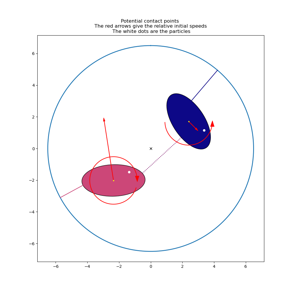
ax.set_title(('Potential contact points \n The red arrows give '
'the relative initial speeds \n The white dots are the '
'particles'))
for kk in range(len(TEST1)):
koerper1 = TEST1[kk][1]
epsilon1 = TEST1[kk][2]
laenge = TEST1[kk][0]
x11 = CPh_list_lam[koerper1](*q_list1, *x_list1, *z_list1, a1, b1, RW1,
epsilon1)[0]
x12 = CPhs_list_lam[koerper1](*q_list1, *x_list1, *z_list1, a1, b1, RW1,
laenge, epsilon1)[0]
z11 = CPh_list_lam[koerper1](*q_list1, *x_list1, *z_list1, a1, b1, RW1,
epsilon1)[1]
z12 = CPhs_list_lam[koerper1](*q_list1, *x_list1, *z_list1, a1, b1, RW1,
laenge, epsilon1)[1]
ax.plot([x11, x12], [z11, z12], color=farben[koerper1], linestyle='-')
# find possible collision points between the ellipses
zaehler = -1
TEST3 = []
le_hilfs = []
epsilone_hilfs = []
for i, j in permutations(range(n), r=2):
zaehler += 1
x0 = (1., 1.) # initial guess
args1 = q_list1 + x_list1 + z_list1 + [a1, b1]
epsilon_min = minimize(funce, x0, args1, jac=func_jakob0, tol=1.e-16)
min_eps = epsilon_min.x % (2.*np.pi)
ll_min = funce(min_eps, args1)
TEST3.append([ll_min, i, j, min_eps[0], min_eps[1], zaehler])
le_hilfs.append(ll_min)
epsilone_hilfs.append((min_eps[0], min_eps[1]))
for kk in range(len(TEST3)):
koerper1 = TEST3[kk][1]
koerper2 = TEST3[kk][2]
epsilon1 = TEST3[kk][3]
epsilon2 = TEST3[kk][4]
x11 = CPhe_list_lam(*q_list1, *x_list1, *z_list1, a1, b1,
epsilon1)[koerper1][0]
x12 = CPhe_list_lam(*q_list1, *x_list1, *z_list1, a1, b1,
epsilon2)[koerper2][0]
z11 = CPhe_list_lam(*q_list1, *x_list1, *z_list1, a1, b1,
epsilon1)[koerper1][1]
z12 = CPhe_list_lam(*q_list1, *x_list1, *z_list1, a1, b1,
epsilon2)[koerper2][1]
ax.plot([x11, x12], [z11, z12], color=farben[koerper1], linestyle='dotted')
# plot the initial speeds
ux_np = np.array(ux_list1)
uz_np = np.array(uz_list1)
u_np = np.array(u_list1)
# normalize the initial speed arrows.
groesse = max(np.max(np.abs(ux_np)), np.max(np.abs(uz_np)))
if np.abs(groesse) < 1.e-5:
groesse = 1.
# If I do not multiply with max(a1, b1) the arrows are too short to be
# seen properly
ux_np = ux_np/groesse * 2. * max(a1, b1)
uz_np = uz_np/groesse * 2. * max(a1, b1)
u_np = u_np / np.max(np.abs(u_np))
# plot the linear speed arrows
style = "Simple, tail_width=0.5, head_width=4, head_length=8"
kw = dict(arrowstyle=style, color="red")
for i in range(n):
a11 = patches.FancyArrowPatch(
(x_list1[i], z_list1[i]), (x_list1[i] + ux_np[i], z_list1[i] +
uz_np[i]), **kw)
ax.add_patch(a11)
# plot the curved arrows for the rotational speed
for j, i in enumerate(u_np):
farbe = 'red'
if i >= 0.:
zeit = np.linspace(0., i * 1.9 * np.pi, 100)
xk = 1.5 * b1 * np.cos(zeit) + x_list1[j]
zk = 1.5 * b1 * np.sin(zeit) + z_list1[j]
ax.plot(xk, zk, color=farbe)
ax.arrow(xk[0], zk[0], xk[0] - xk[1], zk[0] - zk[1], shape='full',
lw=0.5, length_includes_head=True, head_width=0.25,
color=farbe)
else:
zeit = np.linspace(2.*np.pi, (1+i) * 1.9 * np.pi, 100)
xk = 1.5 * b1 * np.cos(zeit) + x_list1[j]
zk = 1.5 * b1 * np.sin(zeit) + z_list1[j]
ax.plot(xk, zk, color=farbe)
ax.arrow(xk[0], zk[0], xk[0] - xk[1], zk[0] - zk[1], shape='full',
lw=0.5, length_includes_head=True, head_width=0.25,
color=farbe)
it took 115 rounds to get valid initial conditions
Numerical integration
The integration seems ‘tricky’:
For the minimum distance between ellipses I switch the methods depending on the distance:
If the distance is very small, or negative, I minimize \(\textrm{distance}(\epsilon_i, \epsilon_j, \textrm{parameters}) = |{}^{CPhe_i} \bar r^{CPhe_j}(\epsilon_i, \epsilon_j)|\) This seems to work better in this case than the \(\nabla\) method, wqhich actually fails quite often. However, without the jacobian, minimize(..) did not work well at all.
If the distance is large, I use \(\nabla_{\epsilon_i, \epsilon_j} distance(\epsilon_i, \epsilon_j, parameters) = 0\) to get \(\epsilon_i, \epsilon_j\). However this is only a necessary condition, and it will only converge to a minimum, if the initial guess is close to the minimum. As in this case, the minimum distance depends continuously on the motion of the ellipses, this seems to work fine if the distances are large.
the cut-off between the methods is 0.0002.
In the case of the minimum distance between ellipse and wall, it does not depend continuously on the motion of the ellipse, hence I use scipy’s minimize() here. I believe, this is slow and ‘inaccurate’ - and does not always find the minimum, as can be seen from the plots. I think, this ‘inaccuracy’, and possibly a non continuous dependency of the result on the parameters send the simulation on a ‘wild goose chase’ when solve_ivp tries to improve the accuracy by going back/forth in time and changing the step size. (I came up with this ‘explanation’, since Radau, which normally works very well with my simulations, did not work well at all here.)
As my numerous trials indicated, this integration is very susceptible to initial conditions and parameters. For example (reibung = friction in German):
with reibung1 = 0.25 max_step = \(10^{-4}\) works fine.
with reibung1 = 0.30, I had to use max_step = \(10^{-5}\) to make it work.
intervall = 10.0 # time interval for the integration
schritte = 1000
max_step = 0.0001
# Adapt the arguments so they fit minimize.
def funcw1(x0, args):
kk = args[-1]
args1 = [args[i] for i in range(len(args)-1)]
return min_distanzCPhiwall_lam[kk](*x0, *args1)
def func_jakobw(x0, args):
kk = args[-1]
args1 = [args[i] for i in range(len(args)-1)]
return jakobw_lam[kk](*x0, *args1)
def funce1(x0, args):
zaehler = args[-1]
args1 = [args[i] for i in range(len(args)-1)]
return min_distanzCPheiCPhej_lam[zaehler](*x0, *args1)
def funce1_abs(x0, args):
zaehler = args[-1]
args1 = [args[i] for i in range(len(args)-1)]
return abs(min_distanzCPheiCPhej_lam[zaehler](*x0, *args1))
def funce1didj(x0, args):
zaehler = args[-1]
args1 = [args[i] for i in range(len(args)-1)]
return min_distanzCPheiCPhej_lam1[zaehler](*x0, *args1)
def func_jakob1(x0, args):
zaehler = args[-1]
args1 = [args[i] for i in range(len(args)-1)]
return jakob_lam[zaehler](*x0, *args1).reshape(2)
# transfer the starting values from the previous cell
l_list1 = l_hilfs
epsilon_list1 = epsilon_hilfs
le_list1 = le_hilfs
epsilone_list1 = epsilone_hilfs
y0 = q_list1 + x_list1 + z_list1 + u_list1 + ux_list1 + uz_list1
pL_vals = ([m01, mo1, iYY1, a1, b1, RW1, nue1, nuw1, EYe1, EYw1, ctau1,
reibung1] + l_list1 + le_list1 + epsilon_list1 + epsilone_list1 +
alpha_list1 + beta_list1 + rhodtwall1 + rhodtmax1 + richtung_list1)
pL1_vals = [m01, mo1, iYY1, a1, b1, RW1, nue1, nuw1, EYe1, EYw1, ctau1,
reibung1] + l_list1 + le_list1 + epsilon_list1 + epsilone_list1
pL2_vals = [m01, mo1, iYY1, a1, b1, RW1, nue1, nuw1, EYe1, EYw1, ctau1,
reibung1] + alpha_list1 + beta_list1
print('starting parameters')
for i, j in zip(pL, pL_vals):
print(f'{str(i):<25} = {j}')
print('\n')
times = np.linspace(0, intervall, int(schritte*intervall))
# needed for the energies further down
LAENGEe = []
zeit = []
ellipsee = []
LAENGEw = []
zeitw = []
ellipsew = []
def gradient(t, y, args):
# find the distance of the ellipses from the wall. and also find rhodtwall
LAENGEw1 = []
ellipsew1 = []
for kk in range(n):
x0 = args[12 + n + n*(n-1) + kk]
args1 = [y[i] for i in range(3*n)] + [a1, b1, RW1] + [kk]
if args[12 + kk] < 0.0002:
tol1 = 1.e-16
else:
tol1 = 1.e-10
epsilon_min = minimize(funcw1, x0, args1, jac=func_jakobw, tol=tol1)
min_eps = epsilon_min.x % (2.*np.pi)
ll_min = funcw1(min_eps, args1)
args[12 + kk] = ll_min
args[12 + n + n*(n-1) + kk] = min_eps[0]
LAENGEw1.append(ll_min)
ellipsew1.append(min_eps)
if 0. <= ll_min <= 0.1:
args[12 + 4*n + 2*n*(n-1) + kk] = rhodtwall_lam(*y, *args)[kk]
LAENGEw.append(LAENGEw1)
ellipsew.append(ellipsew1)
zeitw.append(t)
# find possible collision points between the ellipses, and also find
# rhodtmax
zaehler = -1
LAENGEe1 = []
ellipsee1 = []
for _ in range(n*(n-1)):
zaehler += 1
x0 = args[12 + n + n*(n-1) + n + zaehler] # initial guess
args1 = [y[ij] for ij in range(3*n)] + [a1, b1] + [zaehler]
# if the ellipses are very close to each other, I switch to minimize:
#
# - as this does not happen often, it does not slow down the simulation too
# much
# - if the distances are very small, this seems better than the gradient
# method - which is faster
# - without the jacobian it did not work.
#
# Note, that I niminize the 'unsigned' distance
if args[12 + n + zaehler] <= 0.0002:
epsilon_min = minimize(funce1_abs, x0, args1, jac=func_jakob1,
tol=1.e-16)
else:
epsilon_min = root(funce1didj, x0, args1)
min_eps = epsilon_min.x % (2.*np.pi)
ll_min = funce1(min_eps, args1)
LAENGEe1.append(ll_min)
ellipsee1.append((min_eps[0], min_eps[1]))
args[12 + n + zaehler] = ll_min
args[12 + n + n*(n-1) + n + zaehler] = (min_eps[0], min_eps[1])
if 0. <= ll_min <= 0.01:
rhodteiej = rhodtmax_list_lam(*y, *args)[zaehler]
args[12 + 5*n + 2*n*(n-1) + zaehler] = rhodteiej
# If the distance between the contact points becomes very small,
# calculating the direction CPhe_i.pos_from(CPhej) seems to become
# numerically difficult. This allows me to fix the direction once
# the distance is small. Of course, mechanically speaking not correct,
# but since the intervall of 'incorrect directions is very small,
# it should not matter too much.
args_hilfs = [args[12 + n + n*(n-1) + n + zaehler][0],
args[12 + n + n*(n-1) + n + zaehler][1],
*[y[i] for i in range(3*n)], a1, b1]
if ll_min >= 1.e-12:
args[12 + 5*n + 3*n*(n-1) + zaehler] = richtung_lam[
zaehler](*args_hilfs)
# After penetration, the direction has to be reversed to ensure that the
# contact is the force of ellipse_i on ellipse_j
elif ll_min < -1.e-12:
args[12 + 5*n + 3*n*(n-1) + zaehler] = [-richtung_lam[zaehler]
(*args_hilfs)[0],
-richtung_lam[zaehler]
(*args_hilfs)[1]]
else:
pass
LAENGEe.append(LAENGEe1)
zeit.append(t)
ellipsee.append(ellipsee1)
sol = np.linalg.solve(MM_lam(*y, *args), force_lam(*y, *args))
return np.array(sol).T[0]
resultat1 = solve_ivp(gradient, (0., float(intervall)), y0, args=(pL_vals,),
t_eval=times, max_step=max_step)
resultat = resultat1.y.T
print(resultat1.message)
print((f'to calculate an intervall of {intervall:.2f} sec '
f'it made {resultat1.nfev:,} function calls'))
print('shape of resultat', resultat.shape)
starting parameters
m0 = 1.0
mo = 1.0
iYY = 1.25
a = 2.0
b = 1.0
RW = 6.5
nue = 0.28
nuw = 0.28
EYe = 10000000.0
EYw = 10000000.0
ctau = 0.975
reibung = 0.01
l0 = 2.53433996043252
l1 = 1.6300166232524864
le01 = 3.3346613277141035
le10 = 3.3346613277141026
epsilon0 = 2.087757011359624
epsilon1 = 3.387872190808549
(epsilone01, epsilone10) = (np.float64(5.014745193034272), np.float64(0.40593260225101835))
(epsilone10, epsilone01) = (np.float64(0.4059326022494628), np.float64(5.014745193030075))
alpha0 = 0.5
alpha1 = 0.5
beta0 = 0.5
beta1 = 0.5
rhodtwall0 = 1.0
rhodtwall1 = 2.0
rhodtmax01 = 1.0
rhodtmax10 = 1.0
(richtungx0, richtungz1) = (1.0, 0.0)
(richtungx1, richtungz0) = (1.0, 0.0)
The solver successfully reached the end of the integration interval.
to calculate an intervall of 10.00 sec it made 600,068 function calls
shape of resultat (10000, 12)
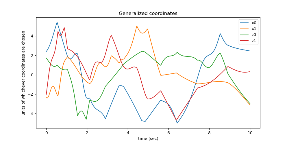
Plot any coordinates you want to see.
N2 = 1000
N1 = max(1, int(resultat.shape[0] / N2))
times1 = []
resultat1 = []
for i in range(resultat.shape[0]):
if i % N1 == 0:
times1.append(times[i])
resultat1.append(resultat[i])
resultat1 = np.array(resultat1)
times1 = np.array(times1)
bezeichnung = (['q' + str(i) for i in range(n)] +
['x' + str(i) for i in range(n)] +
['z' + str(i) for i in range(n)] +
['u' + str(i) for i in range(n)] +
['ux' + str(i) for i in range(n)] +
['uz' + str(i) for i in range(n)])
fig, ax = plt.subplots(figsize=(10, 5))
for i in range(1*n, 3*n):
label = 'gen. coord. ' + str(i)
ax.plot(times1, resultat1[:, i], label=bezeichnung[i])
ax.set_title('Generalized coordinates')
ax.set_xlabel('time (sec)')
ax.set_ylabel('units of whichever coordinates are chosen')
_ = ax.legend()
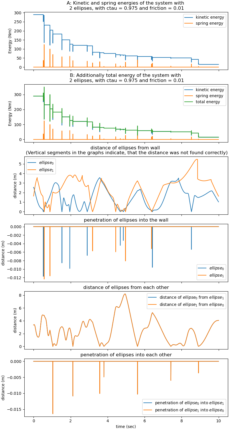
Plot the energies of the system.
If \(c_{\tau} < 1\) or \(reibung \neq 0\), the total energy should drop monotonically. This is due to the Hunt-Crossley prescription of the forces during a collision, due to friction during the collisions respectively.
With \(c_{\tau} = 1\) and \(reibung = 0\), the energy is not constant when two ellipses collide. I do not know, whether there is an error in my program, or whether it is related to the ‘tricky’ integration. With larger \(EY_e\), this error seems to drop. I think, the peaks in the total energy show that I do not catch the correct timings when I plot them. I think so, because the kinetic energy does drop as expected.
schritte = resultat.shape[0]
kin_np = np.empty(schritte)
spring_np = np.empty(schritte)
total_np = np.empty(schritte)
# find the distance of the ellipses from the wall
# find the distances between ellipse
# I try to match the values collected in the integration closely to the times
# given back by the integration.
# argumentw will hold the positions, where this is the case.
argumentw = [0]
zeitw = np.array(zeitw)
for zeit1 in times[: -1]:
start = argumentw[-1]
start1 = np.min(np.argwhere(zeitw >= zeit1))
argumentw.append(start1)
if len(argumentw) != len(times):
raise Exception('Something went wrong')
laengew1 = []
elliw1 = []
for index in argumentw:
laengew1.append(LAENGEw[index])
elliw1.append(ellipsew[index])
# find the distances between ellipse
# I try to match the values collected in the integration closely to the times
# given back by the integration.
# argumente will hold the positions, where this is the case.
argumente = [0]
zeit = np.array(zeit)
for zeit1 in times[: -1]:
start = argumente[-1]
start1 = np.min(np.argwhere(zeit >= zeit1))
argumente.append(start1)
if len(argumente) != len(times):
raise Exception('Something went wrong')
laengee1 = []
ellie1 = []
for index in argumente:
laengee1.append(LAENGEe[index])
ellie1.append(ellipsee[index])
for i in range(schritte):
kin_np[i] = kin_lam(*[resultat[i, j] for j in range(resultat.shape[1])],
*pL2_vals)
spring_np[i] = spring_lam(*[resultat[i, j]
for j in range(resultat.shape[1])],
*[pL_vals[k] for k in range(12)], *laengew1[i],
*elliw1[i], *laengee1[i], *ellie1[i]).squeeze()
total_np[i] = spring_np[i] + kin_np[i]
fig, (ax1, ax2, ax3, ax4, ax5, ax6) = plt.subplots(6, 1, figsize=(8, 15),
layout='constrained',
sharex=True)
for i, j in zip((kin_np, spring_np),
('kinetic energy', 'spring energy')):
ax1.plot(times[: schritte], i, label=j)
ax1.set_ylabel('Energy (Nm)')
ax1.set_title(f'A: Kinetic and spring energies of the system with \n {n} '
f'ellipses, with ctau = {ctau1} and friction = {reibung1}')
ax1.legend()
for i, j in zip((kin_np, spring_np, total_np),
('kinetic energy', 'spring energy', 'total energy')):
ax2.plot(times[: schritte], i, label=j)
ax2.set_ylabel('Energy (Nm)')
ax2.set_title(f'B: Additionally total energy of the system with \n {n} '
f'ellipses, with ctau = {ctau1} and friction = {reibung1}')
ax2.legend()
for koerper in range(n):
laengew1 = np.array(laengew1)
ax3.plot(times, laengew1[:, koerper], label=f'$ellipse_{koerper}$')
ax3.set_title('distance of ellipses from wall \n (Vertical segments '
'in the graphs indicate, that the distance was not found '
'correctly)')
ax3.set_ylabel('distance (m)')
ax3.legend()
for koerper in range(n):
laengew2 = [min(laengew1[jj, koerper], 0.) for jj in range(len(laengew1))]
ax4.plot(times, laengew2, label=f'$ellipse_{koerper}$')
ax4.set_title('penetration of ellipses into the wall')
ax4.set_ylabel('distance (m)')
ax4.legend()
zaehler = -1
for i, j in permutations(range(n), r=2):
zaehler += 1
laengee1 = np.array(laengee1)
ax5.plot(times, laengee1[:, zaehler], label=f'distance of $ellipse_{i}$ '
f'from $ellipse_{j}$')
ax5.set_title('distance of ellipses from each other')
ax5.set_ylabel('distance (m)')
ax5.legend()
zaehler = -1
for i, j in permutations(range(n), r=2):
zaehler += 1
laengee2 = [min(laengee1[jj, zaehler], 0.0) for jj in range(len(laengee1))]
ax6.plot(times, laengee2, label=f'penetration of $ellipse_{i}$ '
f'into $ellipse_{j}$')
ax6.set_title('penetration of ellipses into each other')
ax6.set_xlabel('time (sec)')
ax6.set_ylabel('distance (m)')
_ = ax6.legend()
Animation
As the number of points in time, given as schritte may be verly large, I limit to around zeitpunkte. Otherwise it would take a very long time to finish the animation.
times2 = []
resultat2 = []
zeitpunkte = 200
reduction = max(1, int(resultat.shape[0]/zeitpunkte))
for i in range(resultat.shape[0]):
if i % reduction == 0:
times2.append(times[i])
resultat2.append(resultat[i])
schritte2 = len(times2)
resultat2 = np.array(resultat2)
times2 = np.array(times2)
print('number of points considered:', len(times2))
# X and Z - coordinates of the centers of the ellipses
Dmc_X = np.array([[resultat2[i, j] for j in range(n, 2*n)]
for i in range(schritte2)])
Dmc_Z = np.array([[resultat2[i, j] for j in range(2*n, 3*n)]
for i in range(schritte2)])
Po_X = np.empty((schritte2, n))
Po_Z = np.empty((schritte2, n))
for i in range(schritte2):
Po_X[i] = [Po_pos_lam(*[resultat2[i, j]
for j in range(int(resultat.shape[1]/2.))],
*alpha_list1, *beta_list1, a1, b1)[l1][0]
for l1 in range(n)]
Po_Z[i] = [Po_pos_lam(*[resultat2[i, j]
for j in range(int(resultat.shape[1]/2.))],
*alpha_list1, *beta_list1, a1, b1)[l1][1]
for l1 in range(n)]
# This is to asign colors of 'plasma' to the discs.
Test = mp.colors.Normalize(0, n)
Farbe = mp.cm.ScalarMappable(Test, cmap='plasma')
# color of the starting position
farben = [Farbe.to_rgba(l1) for l1 in range(n)]
def animate_pendulum(times2, Dmc_X, Dmc_Z, Po_X, Po_Z):
fig, ax = plt.subplots(figsize=(8, 8))
ax.axis('on')
theta = np.linspace(0., 2.*np.pi, 200)
aa = RW1 * np.sin(theta)
bb = RW1 * np.cos(theta)
ax.plot(aa, bb, linewidth=2)
LINE1 = []
LINE2 = []
LINE3 = []
LINE4 = []
for i in range(n):
x1 = resultat2[0, n+i]
z1 = resultat2[0, 2*n+i]
elli = patches.Ellipse((x1, z1), width=2.*a1, height=2.*b1,
angle=-np.rad2deg(resultat2[0, i]), zorder=1,
fill=True, color=farben[i], ec='black')
line1 = ax.add_patch(elli)
# the observers
line2, = ax.plot([], [], 'o', markersize=5, color='white',
markeredgecolor='black')
# tracing the centers of the ellipses
line3, = ax.plot([], [], '-', markersize=0, linewidth=0.3)
line4, = ax.plot([], [], 'o', markersize=5, color='yellow',
markeredgecolor='black')
LINE1.append(line1)
LINE2.append(line2)
LINE3.append(line3)
LINE4.append(line4)
def animate(i):
ax.set_title(f'System with {n} bodies, running time {times2[i]:.2f} '
f'sec, $ c_\\tau$ = {ctau1}, friction = {reibung1} \n '
f'The white dots are the particles', fontsize=12)
for j in range(n):
LINE1[j].set_center((resultat2[i, n+j], resultat2[i, 2*n+j]))
LINE1[j].set_angle(-np.rad2deg(resultat2[i, j]))
LINE1[j].set_color(farben[j])
LINE2[j].set_data([Po_X[i, j]], [Po_Z[i, j]])
LINE3[j].set_data([Dmc_X[:i, j]], [Dmc_Z[:i, j]])
LINE3[j].set_color(farben[j])
LINE4[j].set_data(([resultat2[i, n+j]], [resultat2[i, 2*n+j]]))
return LINE1 + LINE2 + LINE3 + LINE4
anim = animation.FuncAnimation(fig, animate, frames=schritte2,
interval=2000*times2.max() / schritte2,
blit=True)
return anim
anim = animate_pendulum(times2, Dmc_X, Dmc_Z, Po_X, Po_Z)
plt.show()