Car hits Points

Objective

• Show how the objective function may be used to force an object to hit preset points along the trajectory, at times determined by opty.

Description

A conventional car is modeled: The rear axle is driven, the front axle does the steering.

No speed possible perpendicular to the wheels.

The car must drive from A to B as fast as possible, and hit four given points along the way.

The car is moving in the horizontal X/Y plane.

Explanation of the Objective Function

• Let \(P_1, P_2, P_3, P_4\) be the four points to be hit, with x and y coordinates \((x_1, y_1), (x_2, y_2), (x_3, y_3), (x_4, y_4)\), and let h be the variable time step size.

• The x - coordinates of the front of the car are given in the array free at the first num_nodes entries, the y - coordinates at the next num_nodes entries.

• One now looks for the entry in the x - coordinates which is closest to, say, \(x_1\). Say, this is the \(m^{th}\) entry, that is it happens at time \(t_m = m \cdot h\). Now calculate \((\textrm{free[m]} - x_1)^2 + (\textrm{free[m + num_nodes]} - y_1)^2\). This is done for all four points.

• The objective function is the sum of these four values, plus free[-1], which holds the time step size \(h\). A weight is applied to the time step size, to determine the relative importance of the closeness to the points and the time step size.

• The gradient of the objective function is calculated accordingly.

Notes

• This method crucially depends on the fact, that opty looks at the complete trajectory simultaneously.

• It is obviously a trade-off between the closeness to the points and the the speed.

• It seems to be quite sensitive, and easily converges to ‘solutions’ which are visually far from being optimal, so this may be a method of last resort only.

States

• \(x, y\) - position of the front of the car

• \(q_0, q_f\) - angle of the car body / steering angle

• \(u_0, u_f\) - angular speed of the car body / steering angle speed

• \(u_x, u_y\) - speed of the front of the car in x and y direction

Inputs

• \(F_b\) - force on the rear axle, driving the car

• \(T_f\) - torque on the front axle, steering the car

Parameters

• \(l\) - length of the car

• \(m_0, m_b, m_f\) - mass of the car body, rear and front axle

• \(i_{ZZ0}, i_{ZZb}, i_{ZZf}\) - inertia of the car body, rear and front axle around the vertical axis

• \(\textrm{reibung}\) - friction coefficient of the rear axle

import sympy.physics.mechanics as me
import numpy as np
import sympy as sm
from scipy.interpolate import CubicSpline

from opty.direct_collocation import Problem
import matplotlib.pyplot as plt
from matplotlib.animation import FuncAnimation

Equations of Motion, Kane’s Method

N, A0, Ab, Af = sm.symbols('N A0 Ab Af', cls=me.ReferenceFrame)
t = me.dynamicsymbols._t
O, Pb, Dmc, Pf = sm.symbols('O Pb Dmc Pf', cls=me.Point)
O.set_vel(N, 0)

q0, qf = me.dynamicsymbols('q_0 q_f')
u0, uf = me.dynamicsymbols('u_0 u_f')
x, y = me.dynamicsymbols('x y')
ux, uy = me.dynamicsymbols('u_x u_y')
Tf, Fb = me.dynamicsymbols('T_f F_b')

reibung = sm.symbols('reibung')

l, m0, mb, mf, iZZ0, iZZb, iZZf = sm.symbols('l m0 mb mf iZZ0, iZZb, iZZf')

A0.orient_axis(N, q0, N.z)
A0.set_ang_vel(N, u0 * N.z)

Ab.orient_axis(A0, 0, N.z)

Af.orient_axis(A0, qf, N.z)
rot = Af.ang_vel_in(N)
Af.set_ang_vel(N, uf * N.z)
rot1 = Af.ang_vel_in(N)

Pf.set_pos(O, x * N.x + y * N.y)
Pf.set_vel(N, ux * N.x + uy * N.y)

Pb.set_pos(Pf, -l * A0.y)
Pb.v2pt_theory(Pf, N, A0)

Dmc.set_pos(Pf, -l/2 * A0.y)
Dmc.v2pt_theory(Pf, N, A0)

# No speed perpendicular to the wheels
vel1 = me.dot(Pb.vel(N), Ab.x) - 0
vel2 = me.dot(Pf.vel(N), Af.x) - 0

I0 = me.inertia(A0, 0, 0, iZZ0)
body0 = me.RigidBody('body0', Dmc, A0, m0, (I0, Dmc))
Ib = me.inertia(Ab, 0, 0, iZZb)
bodyb = me.RigidBody('bodyb', Pb, Ab, mb, (Ib, Pb))
If = me.inertia(Af, 0, 0, iZZf)
bodyf = me.RigidBody('bodyf', Pf, Af, mf, (If, Pf))
BODY = [body0, bodyb, bodyf]


# Forces
FL = [(Pb, Fb * Ab.y), (Af, Tf * N.z), (Dmc, -reibung * Dmc.vel(N))]

kd = sm.Matrix([ux - x.diff(t), uy - y.diff(t), u0 - q0.diff(t),
                me.dot(rot1 - rot, N.z)])
speed_constr = sm.Matrix([vel1, vel2])

q_ind = [x, y, q0, qf]
u_ind = [u0, uf]
u_dep = [ux, uy]

KM = me.KanesMethod(
    N,
    q_ind=q_ind,
    u_ind=u_ind,
    kd_eqs=kd,
    u_dependent=u_dep,
    velocity_constraints=speed_constr,
)

fr, frstar = KM.kanes_equations(BODY, FL)
eom = fr + frstar
eom = kd.col_join(eom)
eom = eom.col_join(speed_constr)
print(f'eom too large to print out. Its shape is {eom.shape} and it has ' +
      f'{sm.count_ops(eom)} operations')

eom too large to print out. Its shape is (8, 1) and it has 428 operations

Set Up the Optimization Problem and Solve It

state_symbols = [x, y, q0, qf, ux, uy, u0, uf]

h = sm.symbols('h')
num_nodes = 100
t0, tf = 0 * h, (num_nodes - 1) * h
interval_value = h

# Specify the known system parameters.
par_map = {}
par_map[m0] = 1.0
par_map[mb] = 0.5
par_map[mf] = 0.5
par_map[iZZ0] = 1.
par_map[iZZb] = 0.5
par_map[iZZf] = 0.5
par_map[l] = 3.0
par_map[reibung] = 0.25

# Coordinates of points to be reached on the journey
points = [8.0, 16.0, 24.0, 32.0]
x1, x2, x3, x4 = points
y1, y2, y3, y4 = [(-1)**j * 30.0 / np.pi * np.sin(np.pi / 40.0 * i)
                  for j, i in enumerate(points)]


def proximity_to_points(free):
    """
    Find the time, where the x - coordinate is closest to the given points,
    and return the sum of the squared distances to the points.
    """
    X1 = (free[0: num_nodes] - x1)**2
    X2 = (free[0: num_nodes] - x2)**2
    X3 = (free[0: num_nodes] - x3)**2
    X4 = (free[0: num_nodes] - x4)**2

    Y1 = (free[num_nodes: 2 * num_nodes] - y1)**2
    Y2 = (free[num_nodes: 2 * num_nodes] - y2)**2
    Y3 = (free[num_nodes: 2 * num_nodes] - y3)**2
    Y4 = (free[num_nodes: 2 * num_nodes] - y4)**2

    minx1 = np.argmin(X1)
    minx2 = np.argmin(X2)
    minx3 = np.argmin(X3)
    minx4 = np.argmin(X4)
    return (X1[minx1] + X2[minx2] + X3[minx3] + X4[minx4] + Y1[minx1] +
            Y2[minx2] + Y3[minx3] + Y4[minx4])


instance_constraints = (
    x.func(t0),
    y.func(t0),
    ux.func(t0),
    uy.func(t0),
    q0.func(t0) + np.pi / 4.0,
    u0.func(t0),
    x.func(tf) - 40.0,
    y.func(tf),
    ux.func(tf),
    uy.func(tf),
)

# Set up the bounds for the optimization variables.
limit = 25.0
bounds = {
    h: (0.0, 0.5),
    x: (-5.0, 45.0),
    y: (-20.0, 20.0),
    qf: (-np.pi / 4.0, np.pi / 4.0),  # limit the steering angle.
    Fb: (-limit, limit),
    Tf: (-limit, limit),
}

# Set up the objective function and its gradient as explained above.

initial_guess = np.ones(10 * num_nodes + 1) * 0.01

# Iterate from a simpler problem -more weight on the speed- to coming closer
# to the points.
for i in range(5):
    # the larger weight, the more the speed is penalized, the less the
    # closeness to the points is important.
    weight = 1.e5 / 10**i

    # Set up the objective function and its gradient as explained above.
    def obj(free):
        return proximity_to_points(free) + free[-1] * weight

    def obj_grad(free):
        X1 = (free[0: num_nodes] - x1)**2
        X2 = (free[0: num_nodes] - x2)**2
        X3 = (free[0: num_nodes] - x3)**2
        X4 = (free[0: num_nodes] - x4)**2
        minx1 = np.argmin(X1)
        minx2 = np.argmin(X2)
        minx3 = np.argmin(X3)
        minx4 = np.argmin(X4)

        grad = np.zeros_like(free)
        grad[minx1] = 2 * (free[minx1] - x1)
        grad[minx2] = 2 * (free[minx2] - x2)
        grad[minx3] = 2 * (free[minx3] - x3)
        grad[minx4] = 2 * (free[minx4] - x4)
        grad[minx1 + num_nodes] = 2 * (free[minx1 + num_nodes] - y1)
        grad[minx2 + num_nodes] = 2 * (free[minx2 + num_nodes] - y2)
        grad[minx3 + num_nodes] = 2 * (free[minx3 + num_nodes] - y3)
        grad[minx4 + num_nodes] = 2 * (free[minx4 + num_nodes] - y4)
        grad[-1] = 1.0 * weight
        return grad

    # Set up the objective function and its gradient as explained above.
    prob = Problem(
        obj,
        obj_grad,
        eom,
        state_symbols,
        num_nodes,
        interval_value,
        known_parameter_map=par_map,
        instance_constraints=instance_constraints,
        bounds=bounds,
    )

    prob.add_option('max_iter', 6000)
    # Find the optimal solution.
    solution, info = prob.solve(initial_guess)
    initial_guess = solution
    print(f'{i+1} - th iteration')
    print('message from optimizer:', info['status_msg'])
    print('Iterations needed', len(prob.obj_value))
    print(f"objective value {info['obj_val']:.3e}")
    print((f"Distance to points {np.sqrt(proximity_to_points(solution)):.3e}"
           f" \n"))

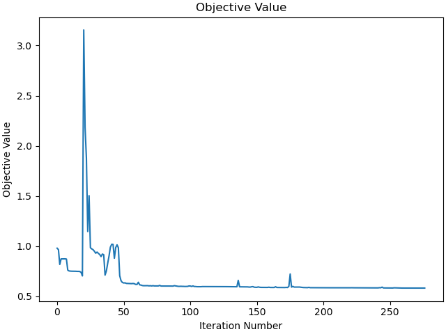
_ = prob.plot_objective_value()

1 - th iteration
message from optimizer: b'Algorithm terminated successfully at a locally optimal point, satisfying the convergence tolerances (can be specified by options).'
Iterations needed 1558
objective value 3.845e+03
Distance to points 1.382e+01

2 - th iteration
message from optimizer: b'Algorithm terminated successfully at a locally optimal point, satisfying the convergence tolerances (can be specified by options).'
Iterations needed 3204
objective value 4.821e+02
Distance to points 8.535e+00

3 - th iteration
message from optimizer: b'Algorithm terminated successfully at a locally optimal point, satisfying the convergence tolerances (can be specified by options).'
Iterations needed 2573
objective value 5.496e+01
Distance to points 1.144e+00

4 - th iteration
message from optimizer: b'Algorithm terminated successfully at a locally optimal point, satisfying the convergence tolerances (can be specified by options).'
Iterations needed 34
objective value 7.633e+00
Distance to points 4.900e-01

5 - th iteration
message from optimizer: b'Algorithm terminated successfully at a locally optimal point, satisfying the convergence tolerances (can be specified by options).'
Iterations needed 277
objective value 5.817e-01
Distance to points 1.715e-02

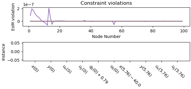
Plot the constraint violations.

_ = prob.plot_constraint_violations(solution)

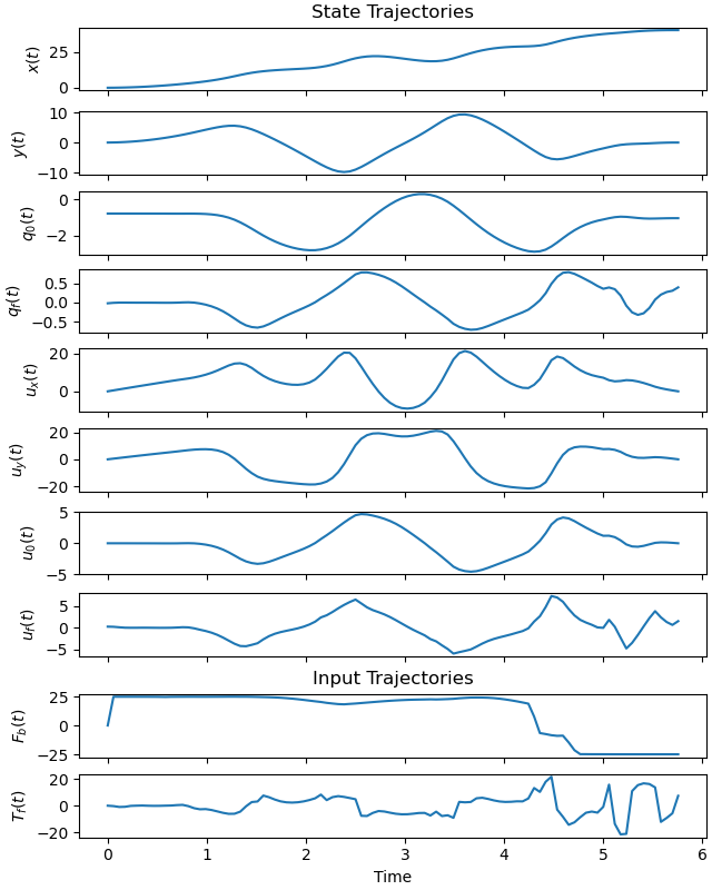
Plot generalized coordinates / speeds and forces / torques

_ = prob.plot_trajectories(solution)

Animation

fps = 15


def add_point_to_data(line, x, y):
    # to trace the path of the point. Copied from Timo.
    old_x, old_y = line.get_data()
    line.set_data(np.append(old_x, x), np.append(old_y, y))


state_vals, input_vals, _, h_val = prob.parse_free(solution)
t_arr = np.linspace(t0, (num_nodes - 1) * h_val, num_nodes)
state_sol = CubicSpline(t_arr, state_vals.T)
input_sol = CubicSpline(t_arr, input_vals.T)

# create additional points for the axles
Pbl, Pbr, Pfl, Pfr = sm.symbols('Pbl Pbr Pfl Pfr', cls=me.Point)

# end points of the force, length of the axles
Fbq = me.Point('Fbq')
la = sm.symbols('la')
fb, tq = sm.symbols('f_b, t_q')

Pbl.set_pos(Pb, -la/2 * Ab.x)
Pbr.set_pos(Pb, la/2 * Ab.x)
Pfl.set_pos(Pf, -la/2 * Af.x)
Pfr.set_pos(Pf, la/2 * Af.x)

Fbq.set_pos(Pb, fb * Ab.y)

coordinates = Pb.pos_from(O).to_matrix(N)
for point in (Dmc, Pf, Pbl, Pbr, Pfl, Pfr, Fbq):
    coordinates = coordinates.row_join(point.pos_from(O).to_matrix(N))

pL, pL_vals = zip(*par_map.items())
la1 = par_map[l] / 1.5                      # length of an axle
coords_lam = sm.lambdify((*state_symbols, fb, *pL, la), coordinates,
                         cse=True)


def init():
    xmin = np.min(state_vals[0, :]) - 3.0
    xmax = np.max(state_vals[0, :]) + 3.0
    ymin = np.min(state_vals[1, :]) - 3.0
    ymax = np.max(state_vals[1, :]) + 3.0

    fig = plt.figure(figsize=(8, 8))
    ax = fig.add_subplot(111)
    ax.set_xlim(xmin, xmax)
    ax.set_ylim(ymin, ymax)
    ax.set_aspect('equal')
    ax.grid()

    ax.scatter([x1, x2, x3, x4], [y1, y2, y3, y4], color='black', marker='o',
               s=25)
    ax.scatter(0.0, 0.0, color='red', marker='o', s=25)
    ax.scatter(40.0, 0.0, color='green', marker='o', s=25)

    line1, = ax.plot([], [], color='orange', lw=2)
    line2, = ax.plot([], [], color='red', lw=2)
    line3, = ax.plot([], [], color='magenta', lw=2)
    line4 = ax.quiver([], [], [], [], color='green', scale=150,
                      width=0.004, headwidth=8)
    line5, = ax.plot([], [], color='blue', lw=0.5)

    return fig, ax, line1, line2, line3, line4, line5


# Function to update the plot for each animation frame
fig, ax, line1, line2, line3, line4, line5 = init()


def update(t):
    message = (f'running time {t:.2f} sec \n The rear axle is red, the ' +
               'front axle is magenta \n The driving/breaking force is green')
    ax.set_title(message, fontsize=12)

    coords = coords_lam(*state_sol(t), input_sol(t)[0], *pL_vals, la1)

    #   Pb, Dmc, Pf, Pbl, Pbr, Pfl, Pfr, Fbq
    line1.set_data([coords[0, 0], coords[0, 2]], [coords[1, 0], coords[1, 2]])
    line2.set_data([coords[0, 3], coords[0, 4]], [coords[1, 3], coords[1, 4]])
    line3.set_data([coords[0, 5], coords[0, 6]], [coords[1, 5], coords[1, 6]])
    add_point_to_data(line5, coords[0, 2], coords[1, 2])

    line4.set_offsets([coords[0, 0], coords[1, 0]])
    line4.set_UVC(coords[0, 7] - coords[0, 0], coords[1, 7] - coords[1, 0])
    # return line1, line2, line3, line4, #line5, line6,


tf = (num_nodes - 1) * h_val
frames = np.linspace(t0, tf, int(fps * (tf - t0)))
animation = FuncAnimation(fig, update, frames=frames, interval=1000 / fps)

plt.show()

Once Loop Reflect

WARNING:matplotlib.animation:MovieWriter ffmpeg unavailable; using Pillow instead.