Note
Go to the end to download the full example code.
Particle in Changing Environment
Objective
Show how it is possible to change the equations of motion during the motion using smooth hump functions.
Description
A particle is moving along a street defined by a sine function from 0.0 m to 20.0 m in the x direction as fast as possible.
The particle has a rocket engine that provides thrust. The particle’s mass changes during the motion, as does the friction acting on it and the exhaust speed. This is very artificial, of course, just to show how it can be done.
So, in a way the equations of motion change during the motion.
Notes
Even with this simple example, one has to ‘play around’ a bit to get results. For example, if the steepness of the hump functions is too high, one gets seemingly unreasonable results.
Very strange: If \(T\) is included as a
state, the optimization works fine. If it is made aninput, the result is very different, much less reasonable. No idea why.
States
\(x\) : x position of the particle
\(y\) : y position of the particle
\(q\) : direction of the force/thrust
\(u_x\) : x velocity of the particle
\(u_y\) : y velocity of the particle
\(u\) : angular velocity of the direction of the force/thrust
\(m\) : mass of the fuel
\(T\) : Torque to change the direction of the thrust, of no importance
Inputs
\(\alpha\) : burn rate of the fuel: \(\dot{m} = - \alpha m\)
Parameters
\(x_1, x_2, x_3\) : positions along the street where the changes happen
\(a, b\) : parameters defining the street shape
\(v_{gas}\) : exhaust speed of the rocket engine
\(m_0\) : payload mass (net weight without fuel )
import numpy as np
import matplotlib.pyplot as plt
import sympy as sm
import sympy.physics.mechanics as me
from opty import Problem
from scipy.interpolate import CubicSpline
from matplotlib.patches import FancyArrowPatch
from matplotlib.animation import FuncAnimation
Equations of Motion
N, A = me.ReferenceFrame('N'), me.ReferenceFrame('A')
O, P = me.Point('O'), me.Point('P')
O.set_vel(N, 0)
t = me.dynamicsymbols._t
steep = sm.symbols('steep')
steepness = 5.0
x1, x2, x3 = sm.symbols('x1 x2 x3')
a, b = sm.symbols('a b')
x, y, ux, uy, q, u = me.dynamicsymbols('x y ux uy q u')
m, mdt = me.dynamicsymbols('m mdt')
alpha = me.dynamicsymbols('alpha')
v_gas = sm.symbols('v_gas')
m0 = sm.symbols('m0')
mu = sm.symbols('mu')
T = me.dynamicsymbols('T')
def strasse(x, a, b):
return a * sm.sin(b * x)
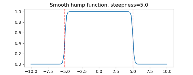
Define the smooth hump function, and plot it.
def smooth_hump(x, x1, x2, steepness):
return 0.5 * (sm.tanh(steepness * (x - x1)) -
sm.tanh(steepness * (x - x2)))
hump_lambda = sm.lambdify((x, x1, x2, steep),
smooth_hump(x, x1, x2, steep), cse=True)
xx = np.linspace(-10, 10, 100)
fig, ax = plt.subplots(figsize=(6.4, 2.5))
ax.plot(xx, hump_lambda(xx, -5, 5, steepness))
ax.axvline(-5, color='red', linestyle='--')
ax.axvline(5, color='red', linestyle='--')
_ = ax.set_title('Smooth hump function, steepness={}'.format(steepness))
Define the particle system.
A.orient_axis(N, q, N.z)
A.set_ang_vel(N, u * N.z)
P.set_pos(O, x * N.x + y * N.y)
P.set_vel(N, ux * N.x + uy * N.y)
Between x1 and x2 the mass of the payload increases from \(m + m_0\) to \(m + 4 m_0\).
Pa = me.Particle('Pa', P, m + m0 + 3*m0 * smooth_hump(x, x1, x2, steepness))
Friction and exhaust speed change between x2 and x3
forces = [(P, -m.diff(t) *
(v_gas - 0.5 * v_gas * smooth_hump(x, x2, x3, steepness)) * A.x -
(mu + 5.0 * mu * smooth_hump(x, x2, x3, steepness)) *
(ux * N.x + uy * N.y)),
(A, T * N.z - 0.01 * u * N.z)]
Set up Kane’s Method and get the equations of motion.
kd = sm.Matrix([
x.diff(t) - ux,
y.diff(t) - uy,
q.diff(t) - u,
])
kane = me.KanesMethod(
N,
q_ind=[x, y, q],
u_ind=[ux, uy, u],
kd_eqs=kd
)
fr, frstar = kane.kanes_equations([Pa], forces)
eom = kd.col_join(fr + frstar)
Add the fuel consumption equation. The assumption is, that the the exhaust is proportional to the fuel left: \(\dfrac{dm(t)}{dt} = - \alpha m(t)\)
eom = eom.col_join(sm.Matrix([m.diff(t) + alpha * m]))
Particle to stay on the street.
mdt - m.diff(t) is added, so m.diff(t) is available and the force may be calculated for the animation.
eom = eom.col_join(sm.Matrix([y - strasse(x, a, b), mdt - m.diff(t)]))
Set Up the Optimization
h = sm.symbols('h')
num_nodes = 201
t0, tb, tf = 0.0, h * int((num_nodes - 1)/2), h * (num_nodes - 1)
interval = h
state_symbols = (x, y, q, ux, uy, u, m, T)
instance_constraint = (
x.func(t0),
y.func(t0),
q.func(t0),
ux.func(t0),
uy.func(t0),
u.func(t0),
m.func(t0) - 5.0,
ux.func(tb) - 0.0,
uy.func(tb) - 0.0,
x.func(tf) - 20.0,
ux.func(tf) - 0.0,
uy.func(tf) - 0.0,
)
bounds = {
h: (0.0, 1.0),
alpha: (0.0, 0.5),
T: (-5.0, 5.0),
q: (-np.pi, np.pi),
x: (0.0, 20.0),
}
Keep the particle on the street, within + / - 0.5 units.
eom_bounds = {7: (-0.5, 0.5)}
Define the known parameters, the objective function and the Problem.
par_map = {
x1: 5.0,
x2: 10.0,
x3: 15.0,
m0: 1.0,
a: 2.0,
b: np.pi / 10,
v_gas: 100.0,
mu: 1.0,
}
def obj(free):
return free[-1]
def obj_grad(free):
grad = np.zeros_like(free)
grad[-1] = 1.0
return grad
prob = Problem(
obj,
obj_grad,
eom,
state_symbols,
num_nodes,
interval,
known_parameter_map=par_map,
instance_constraints=instance_constraint,
bounds=bounds,
eom_bounds=eom_bounds,
backend='cython',
time_symbol=t,
)
Solve the problem.
prob.add_option('max_iter', 5000)
initial_guess = np.ones(prob.num_free) * 0.1
for _ in range(1):
solution, info = prob.solve(initial_guess)
initial_guess = solution
print(info['status_msg'])
b'Algorithm terminated successfully at a locally optimal point, satisfying the convergence tolerances (can be specified by options).'
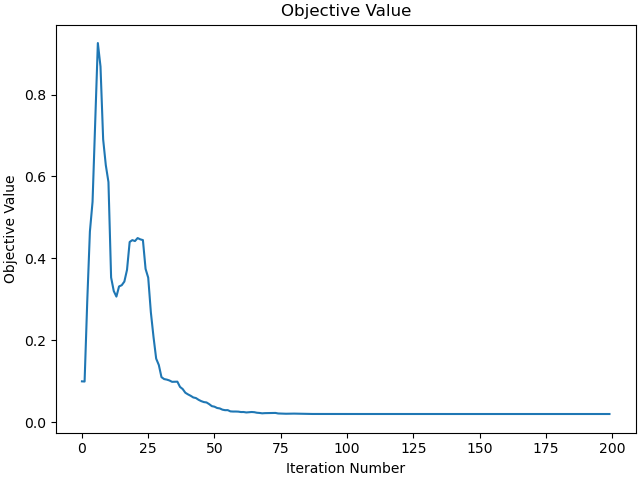
Plot the objective value.
_ = prob.plot_objective_value()
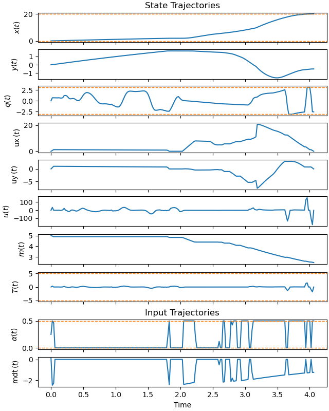
Plot the trajectories.
_ = prob.plot_trajectories(solution, show_bounds=True)
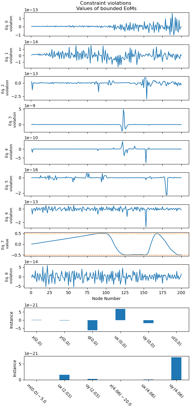
Plot the constraint violations.
_ = prob.plot_constraint_violations(solution, show_bounds=True,
subplots=True)
Animation
fps = 25
street_lam = sm.lambdify((x, a, b), strasse(x, a, b))
state_vals, input_vals, _, h_val = prob.parse_free(solution)
tf = h_val * (num_nodes - 1)
kraft_vals = input_vals.T[:, 0] * input_vals.T[:, 1]
t_arr = np.linspace(t0, tf, num_nodes)
state_sol = CubicSpline(t_arr, state_vals.T)
input_sol = CubicSpline(t_arr, input_vals.T)
kraft_sol = CubicSpline(t_arr, kraft_vals)
# create additional point for the force
Pf = sm.symbols('Pf', cls=me.Point)
kraft = sm.symbols('kraft')
Pf.set_pos(P, kraft * A.x)
coordinates = P.pos_from(O).to_matrix(N)
coordinates = coordinates.row_join(Pf.pos_from(P).to_matrix(N))
pL, pL_vals = zip(*par_map.items())
coords_lam = sm.lambdify((*state_symbols, kraft, *pL), coordinates,
cse=True)
def init():
xmin, xmax = -1.0, 21.0
ymin, ymax = -par_map[a]-1.0, par_map[a]+1.0
fig = plt.figure(figsize=(8, 8))
ax = fig.add_subplot(111)
ax.set_xlim(xmin, xmax)
ax.set_ylim(ymin, ymax)
ax.set_aspect('equal')
ax.grid()
XX = np.linspace(xmin, xmax, 200)
ax.plot(XX, street_lam(XX, par_map[a],
par_map[b]) + 0.5, color='black', linestyle='-')
ax.plot(XX, street_lam(XX, par_map[a],
par_map[b]) - 0.5, color='black', linestyle='-')
ax.axvline(par_map[x1], color='red', linestyle='--')
ax.axvline(par_map[x2], color='red', linestyle='--')
ax.axvline(par_map[x3], color='red', linestyle='--')
ax.set_xlabel('x position [m]')
ax.set_ylabel('y position [m]')
arrow0 = FancyArrowPatch(
posA=(6, -5.5),
posB=(7.5, -1),
arrowstyle='->', # arrow head
connectionstyle='arc3,rad=-0.3',
color='blue',
mutation_scale=20,
lw=0.5,
)
ax.add_patch(arrow0)
ax.text(5.0, -5.5, f"Here the mass \njumps from $m(t) + m_0$ to "
"$m(t) + 4 m_0$",
fontsize=8, color='blue')
ax.fill_between(
[par_map[x1], par_map[x2]],
y1=ax.get_ylim()[0],
y2=ax.get_ylim()[1],
hatch='//',
facecolor='none', # important: no solid fill
edgecolor='blue',
alpha=0.5
)
arrow1 = FancyArrowPatch(
posA=(15, -5.5),
posB=(12.5, -1),
arrowstyle='->', # arrow head
connectionstyle='arc3,rad=-0.3',
color='red',
mutation_scale=20,
lw=0.5,
)
ax.add_patch(arrow1)
ax.text(12.5, -5.5, f"Here the friction \njumps from $\\mu$ to 6$\\mu$ \n"
f"the exhaust speed drops 50%",
fontsize=8, color='red')
ax.fill_between(
[par_map[x2], par_map[x3]],
y1=ax.get_ylim()[0],
y2=ax.get_ylim()[1],
hatch='\\',
facecolor='none', # important: no solid fill
edgecolor='red',
alpha=0.5,
)
line1 = ax.scatter([], [], color='red', s=100)
pfeil = ax.quiver([], [], [], [], color='green', scale=5, width=0.004,
headwidth=8)
return fig, ax, line1, pfeil
# Function to update the plot for each animation frame
fig, ax, line1, pfeil = init()
def update(t):
message = (f'running time {t:.2f} sec \n '
'The driving/breaking force is green')
ax.set_title(message, fontsize=12)
coords = coords_lam(*state_sol(t), -kraft_sol(t), *pL_vals)
line1.set_offsets([coords[0, 0], coords[1, 0]])
pfeil.set_offsets([coords[0, 0], coords[1, 0]])
pfeil.set_UVC(coords[0, 1], coords[1, 1])
frames = np.linspace(t0, tf, int(fps * (tf - t0)))
animation = FuncAnimation(fig, update, frames=frames, interval=2000 / fps)
plt.show()
Total running time of the script: (0 minutes 25.084 seconds)