Mixed State-Control Constraints (betts-10-113)

This is example 10.113 from John T. Betts, Practical Methods for Optimal Control Using NonlinearProgramming, 3rd edition, Chapter 10: Test Problems.

More details are in section 4.14, example 4.10 of the book.

States

• \(y_1, y_2\) : state variables

Controls

• \(u\) : control variable

import numpy as np
import sympy as sm
import sympy.physics.mechanics as me
import time
from opty.direct_collocation import Problem
from opty.utils import create_objective_function, MathJaxRepr

Equations of Motion

t = me.dynamicsymbols._t

# Parameter
p = 0.14

y1, y2 = me.dynamicsymbols('y1, y2')
u = me.dynamicsymbols('u')

eom = sm.Matrix([
    -y1.diff(t) + y2,
    -y2.diff(t) - y1 + y2*(1.4 - p * y2**2) + 4 * u,
    u + y1/6
])

MathJaxRepr(eom)

$$\left[\begin{matrix}y_{2} - \dot{y}_{1}\\\left(1.4 - 0.14 y_{2}^{2}\right) y_{2} + 4 u - y_{1} - \dot{y}_{2}\\u + \frac{y_{1}}{6}\end{matrix}\right]$$

Define and Solve the Optimization Problem

num_nodes = 10001
t0, tf = 0.0, 4.5
interval_value = (tf - t0) / (num_nodes - 1)

state_symbols = (y1, y2)
unkonwn_input_trajectories = (u,)

Specify the objective function and form the gradient.

objective = sm.Integral(u**2 + y1**2, t)

obj, obj_grad = create_objective_function(
    objective,
    state_symbols,
    unkonwn_input_trajectories,
    tuple(),
    num_nodes,
    interval_value
)

instance_constraints = (
    y1.func(t0) + 5,
    y2.func(t0) + 5,
)

Bound for the algebraic eom.

eom_bounds = {2: (-np.inf, 0.0)}

Set up Problem

prob = Problem(
    obj,
    obj_grad,
    eom,
    state_symbols,
    num_nodes,
    interval_value,
    instance_constraints=instance_constraints,
    eom_bounds=eom_bounds,
    time_symbol=t,
)

Rough initial guess

initial_guess = np.ones(prob.num_free) * 0.1

Find the optimal solution.

start = time.time()
solution, info = prob.solve(initial_guess)
print(f"Solved in {time.time() - start:.2f} seconds.")
print(info['status_msg'])
Jstar = 44.8044433
print(f"Objective value achieved: {info['obj_val']:.4f}, as per the book "
      f"it is {Jstar}, so the difference to the value in the book is: "
      f"{(-info['obj_val'] + Jstar) / Jstar * 100:.3f} % ")

Solved in 3.68 seconds.
b'Algorithm terminated successfully at a locally optimal point, satisfying the convergence tolerances (can be specified by options).'
Objective value achieved: 44.7911, as per the book it is 44.8044433, so the difference to the value in the book is: 0.030 %

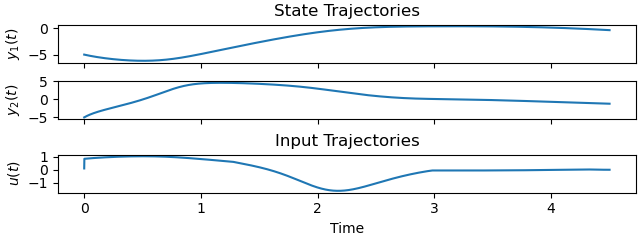
Plot the optimal state and input trajectories.

_ = prob.plot_trajectories(solution)

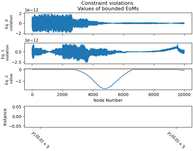
Plot the constraint violations.

_ = prob.plot_constraint_violations(solution, subplots=True, show_bounds=True)

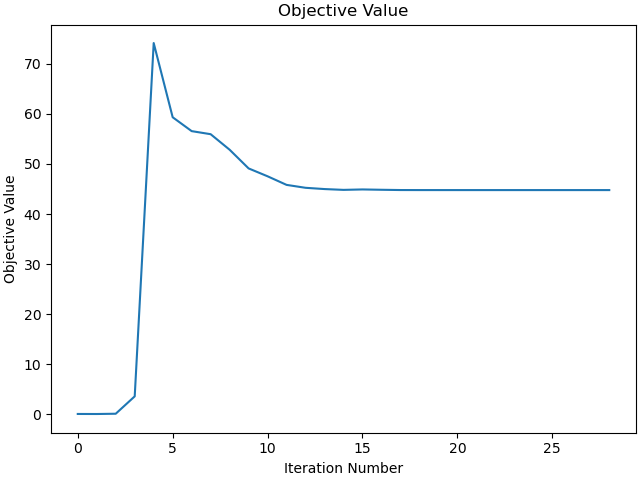
Plot the objective function.

_ = prob.plot_objective_value()