Free-Flying Robot (betts_10_43)

This is example 10.43 from Betts, Practical Methods for Optimal Control Using NonlinearProgramming, 3rd edition, Chapter 10: Test Problems.

More details are in chapter 8.13, example 8.17 of this book.

States

• \(y_0, ...y_5\): state variables

Specifieds

• \(u_0, ..., u_3\) : control variables

import numpy as np
import sympy as sm
import sympy.physics.mechanics as me
import time
from opty import Problem
from opty.utils import create_objective_function, MathJaxRepr

Equations of motion.

t = me.dynamicsymbols._t
y = me.dynamicsymbols(f'y:{6}')
u = me.dynamicsymbols(f'u:{4}')
uy = [y[i].diff(t) for i in range(6)]

alpha, beta = sm.symbols('alpha beta', real=True)

eom = sm.Matrix([
    -uy[0] + y[3],
    -uy[1] + y[4],
    -uy[2] + y[5],
    -uy[3] + (u[0]-u[1]+u[2]-u[3]) * sm.cos(y[2]),
    -uy[4] + (u[0]-u[1]+u[2]-u[3]) * sm.sin(y[2]),
    -uy[5] + alpha*(u[0]-u[1]) - beta*(u[2]-u[3]),
    u[0] + u[1],
    u[2] + u[3],
])

MathJaxRepr(eom)

$$\left[\begin{matrix}y_{3} - \dot{y}_{0}\\y_{4} - \dot{y}_{1}\\y_{5} - \dot{y}_{2}\\\left(u_{0} - u_{1} + u_{2} - u_{3}\right) \cos{\left(y_{2} \right)} - \dot{y}_{3}\\\left(u_{0} - u_{1} + u_{2} - u_{3}\right) \sin{\left(y_{2} \right)} - \dot{y}_{4}\\\alpha \left(u_{0} - u_{1}\right) - \beta \left(u_{2} - u_{3}\right) - \dot{y}_{5}\\u_{0} + u_{1}\\u_{2} + u_{3}\end{matrix}\right]$$

Set Up the Optimization Problem and Solve It

t0, tf = 0.0, 12.0
num_nodes = 2001
interval_value = (tf - t0)/(num_nodes - 1)

state_symbols = y
specified_symbols = u

Specify the objective function and form the gradient.

start = time.time()
obj_func = sm.Integral(sum([u[i] for i in range(4)]), t)
obj, obj_grad = create_objective_function(
    obj_func,
    state_symbols,
    specified_symbols,
    tuple(),
    num_nodes,
    node_time_interval=interval_value)

Specify the symbolic instance constraints, the bounds and known parameters.

instance_constraints = (
    y[0].func(t0) + 10.0,
    y[1].func(t0) + 10.0,
    y[2].func(t0) - np.pi/2,
    y[3].func(t0),
    y[4].func(t0),
    y[5].func(t0),
    y[0].func(tf),
    y[1].func(tf),
    y[2].func(tf),
    y[3].func(tf),
    y[4].func(tf),
    y[5].func(tf),
)

bounds = {u[i]: (0.0, 1.0) for i in range(4)}

eom_bounds = {
    6: (-np.inf, 1.0),
    7: (-np.inf, 1.0),
}

par_map = {
    alpha: 0.2,
    beta: 0.2,
}

Create the optimization problem.

prob = Problem(
    obj,
    obj_grad,
    eom,
    state_symbols,
    num_nodes,
    interval_value,
    instance_constraints=instance_constraints,
    known_parameter_map=par_map,
    bounds=bounds,
    eom_bounds=eom_bounds,
    time_symbol=t,
)

Give some rough estimates for the trajectories.

initial_guess = np.zeros(prob.num_free)

Find the optimal solution.

start = time.time()
solution, info = prob.solve(initial_guess)
end = time.time()
print(info['status_msg'])
Jstar = 7.91055654
print(f"Objective value achieved: {info['obj_val']:.4f}, as per the book "
      f"it is {Jstar:.4f}, so the deviation is: "
      f"{(info['obj_val'] - Jstar)/Jstar*100:.3f} % ")
print(f"Time taken for the simulation: {end - start:.2f} s")

b'Algorithm terminated successfully at a locally optimal point, satisfying the convergence tolerances (can be specified by options).'
Objective value achieved: 7.6918, as per the book it is 7.9106, so the deviation is: -2.765 %
Time taken for the simulation: 82.41 s

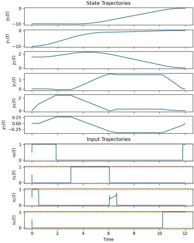
Plot the optimal state and input trajectories.

_ = prob.plot_trajectories(solution, show_bounds=True)

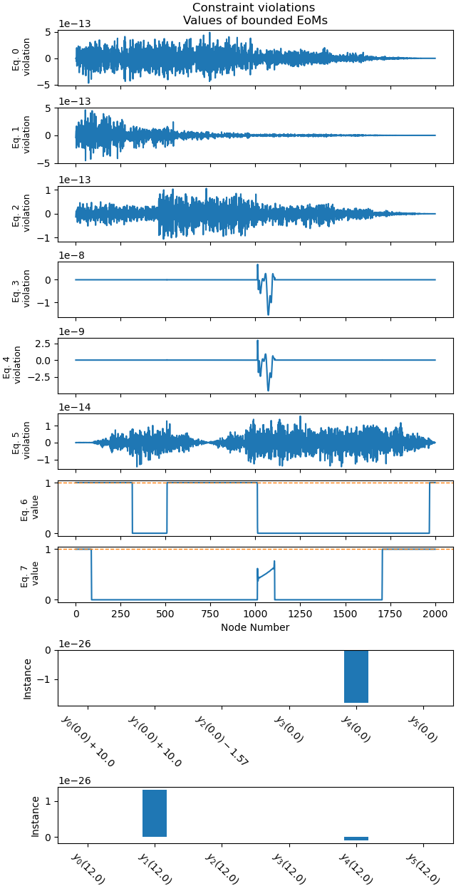
Plot the constraint violations.

_ = prob.plot_constraint_violations(solution, subplots=True, show_bounds=True)

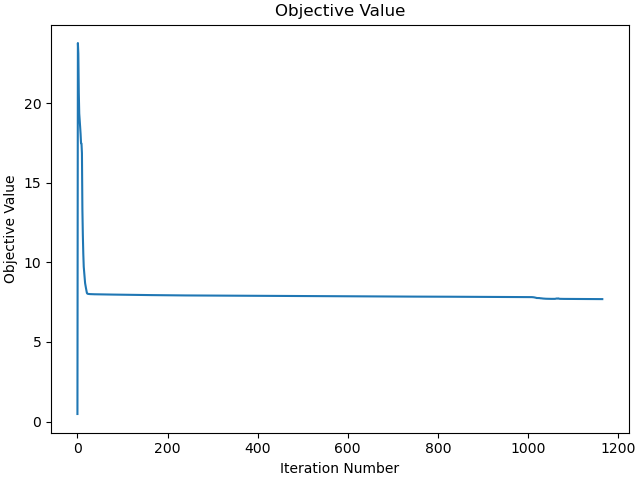
Plot the objective function.

_ = prob.plot_objective_value()