Note
Go to the end to download the full example code.
Axle Rolling on an Uneven Surface
Description
Two thin homogeneous wheels of mass \(m_L, m_R\) and radius \(r_L, r_R\) are attached to a massless axle of length \(l\). They can rotate independently from each other and roll on a smooth surface in the X/Y plane without slipping. The surface is smooth enough that at any point in time the wheels touch the surface at exactly one point. A particle of mass \(m_o\) is attached on the rim of each wheel. Gravity points in the negative Z direction.
Notes
While on a flat surface this system has two degrees of freedom, on a general smooth uneven surface the system has only one degree of freedom.
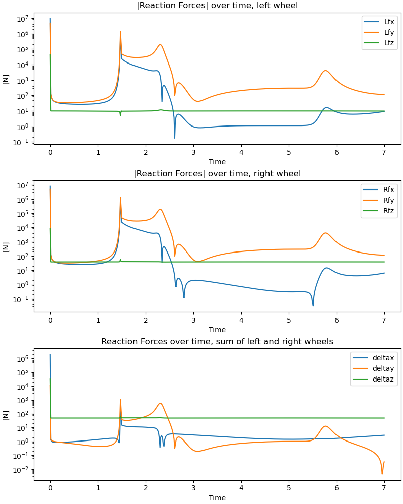
The system is difficult to integrate numerically, it seems to be very stiff. The reaction forces enforcing the no slip condition are very large at some points in time.
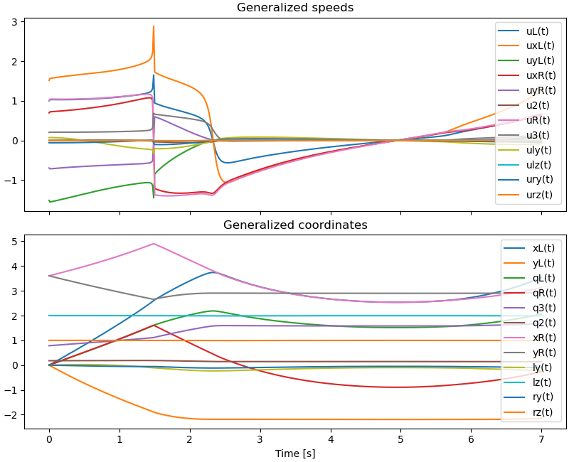
The coordinates of the contact points change (almost) non-differentiably at some times (In the plot below, at around 1.5 sec.)
States
\(q_L, q_R\) : the angles of the wheels w.r.t. the axle.
\(u_L, u_R\) : the speeds of the wheels.
\(x_L, z_L, x_R, z_R\) : the coordinates of the contact points.
\(ux_L, uz_L, ux_R, uz_R\) : the speeds of the contact points.
\(l_y, l_z, r_y, r_z\) : the components of the vectors from the contact points to the centers of mass.
\(ul_y, ul_z, ur_y, ur_z\) : the speeds of these components.
Parameters
\(m_L, m_R, m_o\) : the masses of the wheels and the particles.
\(g\) : the gravitational acceleration.
\(r_L, r_R\) : the radii of the wheels.
\(l\) : the length of the axle.
import sympy as sm
import sympy.physics.mechanics as me
import time
import numpy as np
import matplotlib.pyplot as plt
from scipy.integrate import solve_ivp
from scipy.optimize import root, minimize
from scipy.interpolate import interp1d
from matplotlib.animation import FuncAnimation
from matplotlib.patches import Ellipse
from matplotlib.transforms import Affine2D
Equations of Motion
Rotation angles of the wheels and the body, and their speeds.
qL, qR, q2, q3 = me.dynamicsymbols('qL qR q2 q3')
uL, uR, u2, u3 = me.dynamicsymbols('uL uR u2 u3')
Coordinates of the contact points of the left / right wheel and their speeds.
xL, yL, xR, yR = me.dynamicsymbols('xL yL xR yR')
uxL, uyL, uxR, uyR = me.dynamicsymbols('uxL uyL uxR uyR')
Needed for the noncontributing forces at the contact points.
Lauxx, Lauxy, Lauxz, Rauxx, Rauxy, Rauxz = me.dynamicsymbols(
'Lauxx Lauxy Lauxz Rauxx Rauxy Rauxz')
Lfx, Lfy, Lfz, Rfx, Rfy, Rfz = me.dynamicsymbols(
'Lfx Lfy Lfz Rfx Rfy Rfz')
Components of the vectors from the contact points to the centers of mass, in AX and their speeds.
ly, lz, ry, rz = me.dynamicsymbols('ly lz ry rz')
uly, ulz, ury, urz = me.dynamicsymbols('uly ulz ury urz')
Parameters of the system: masses, gravity, radii of the wheels, and distance between the wheels.
mL, mR, mo, g, rL, rR, l = sm.symbols(
'mL mR mo g rL rR l')
Parameters for the surface.
amplitude, frequenz, reibung, alpha, beta, gamma = sm.symbols(
'amplitude frequenz reibung alpha beta gamma')
Define the reference frames and points.
N, AX, AL, AR = sm.symbols('N, AX, AL, AR', cls=me.ReferenceFrame)
O, CPL, CPR, DmcL, DmcR = sm.symbols('O, CPL, CPR, DmcL, DmcR',
cls=me.Point)
m_DmcL, m_DmcR = sm.symbols('m_DmcL, m_DmcR', cls=me.Point)
O.set_vel(N, 0)
t = me.dynamicsymbols._t
The axle does not rotate around itself.
AX.orient_body_fixed(N, [q3, q2, 0], 'ZYX')
AX.set_ang_vel(N, u2*AX.y + u3*AX.z)
The left wheel rotates around the axle, that is, around AX.x, similarly for the right wheel.
AL.orient_axis(AX, qL, AX.x)
AL.set_ang_vel(AX, uL*AX.x)
AR.orient_axis(AX, qR, AX.x)
AR.set_ang_vel(AX, uR*AX.x)
Particles attached to the wheels.
m_DmcL.set_pos(DmcL, rL*AL.y)
m_DmcR.set_pos(DmcR, rR*AR.y)
The street is modelled. rumpel must be an integer.
x_h, y_h = sm.symbols('x_h y_h')
rumpel = 2
def gesamt(x, y, amplitude, frequenz, rumpel):
strasse = sum([amplitude/j * (sm.sin(j*frequenz*sm.pi * x) +
sm.sin(j*frequenz*sm.pi * y))
for j in range(1, rumpel)])
return strasse
def gesamt_plot(x_h, y_h, amplitude, frequenz):
return sum([amplitude/j * (sm.sin(j*frequenz*sm.pi * x_h) +
sm.sin(j*frequenz*sm.pi * y_h))
for j in range(1, rumpel)])
Create the dictionary to replace \(\dfrac{d}{dt}(\textrm{gen. coord})\) with the corresponding symbols.
kin_dict = {
xL.diff(t): uxL,
yL.diff(t): uyL,
xR.diff(t): uxR,
yR.diff(t): uyR,
qL.diff(t): uL,
qR.diff(t): uR,
ly.diff(t): uly,
lz.diff(t): ulz,
ry.diff(t): ury,
rz.diff(t): urz,
q2.diff(t): u2,
q3.diff(t): u3,
}
CPL is the contact point, where the left wheel touches the street. So its velocity is zero.
CPL.set_pos(O, xL*N.x + yL*N.y +
gesamt(xL, yL, amplitude, frequenz, rumpel)*N.z)
CPL.set_vel(N, Lauxx*N.x + Lauxy*N.y + Lauxz*N.z)
Define the vectors pointing from the contact point to the corresponding center of the wheel. \(vector_L \perp AX.x\) and \(vector_R \perp AX.x\), so they have no component in AX.x direction.
vectorL = ly * AX.y + lz * AX.z
vectorR = ry * AX.y + rz * AX.z
\(vector_L\) and \(vector_R\) must have magnitude equal to the radius of the respective wheel.
constr_length = sm.Matrix([
vectorL.magnitude() - rL,
vectorR.magnitude() - rR,
])
constr_length
Matrix([
[-rL + sqrt(ly(t)**2 + lz(t)**2)],
[-rR + sqrt(ry(t)**2 + rz(t)**2)]])
Set centers of mass of wheels, second contact point CPR.
DmcL.set_pos(CPL, vectorL)
DmcR.set_pos(DmcL, l*AX.x)
CPR.set_pos(DmcR, -vectorR)
Contact point has zero speed.
CPR.set_vel(N, Rauxx*N.x + Rauxy*N.y + Rauxz*N.z)
\(vector_L\) must be in the plane formed by the gradient \(n_L\) at the point (xL, yL) and by AX.x the direction of the axle, that is \(vector_L \circ (n_L \times AX.x) = 0\). Same for \(vector_R\).
nL = (-gesamt(xL, yL, amplitude, frequenz, rumpel).diff(xL) * N.x -
gesamt(xL, yL, amplitude, frequenz, rumpel).diff(yL) * N.y +
N.z).normalize()
nR = (-gesamt(xR, yR, amplitude, frequenz, rumpel).diff(xR) * N.x -
gesamt(xR, yR, amplitude, frequenz, rumpel).diff(yR) * N.y +
N.z).normalize()
perpL = nL.cross(AX.x)
perpR = nR.cross(AX.x)
constrT = sm.Matrix([
perpL.dot(vectorL),
perpR.dot(vectorR),
])
Determine the constraints for \(xR, yR, q_2\) for the location of CPR.
CPR_pos = xR*N.x + yR*N.y + gesamt(xR, yR, amplitude, frequenz, rumpel)*N.z
delta_loc = CPR.pos_from(O) - CPR_pos
constr_CPR = sm.Matrix([
delta_loc.dot(N.x),
delta_loc.dot(N.y),
delta_loc.dot(N.z),
])
Combine the configuration constraints.
config_constr = constr_length.col_join(constrT).col_join(constr_CPR)
print(f"config_constr contains {sm.count_ops(config_constr)} operations "
f"and has shape {config_constr.shape}")
config_constr contains 484 operations and has shape (7, 1)
No slip condition for CPL and for CPR, note that v(CPL) = 0 and v(CPR) = 0.
DmcL.v2pt_theory(CPL, N, AL)
DmcR.v2pt_theory(CPR, N, AR)
vDmcL = DmcL.pos_from(O).diff(t, N)
vDmcR = DmcR.pos_from(O).diff(t, N)
deltaL_vel = vDmcL - DmcL.vel(N)
deltaR_vel = vDmcR - DmcR.vel(N)
frame = N
constr_no_slip = sm.Matrix([
deltaL_vel.dot(frame.x),
deltaL_vel.dot(frame.y),
deltaR_vel.dot(frame.x),
deltaR_vel.dot(frame.y),
])
Now the speeds of DmcL, DmcR are definded, so the speeds of m_DmcL, m_DmcR can be defined as well.
m_DmcL.v2pt_theory(DmcL, N, AL)
_ = m_DmcR.v2pt_theory(DmcR, N, AR)
Combine the speed constraints.
speed_constr = (constr_no_slip.col_join(config_constr.diff(t)))
print(f"speed_constr contains {sm.count_ops(speed_constr):,} operations"
f"and have shape {speed_constr.shape}")
speed_constr contains 2,713 operationsand have shape (11, 1)
Kane’s Equations.
iXXL = 0.5 * mL * rL**2
iYYL = 0.25 * mL * rL**2
iZZL = 0.25 * mL * rL**2
iXXR = 0.5 * mR * rR**2
iYYR = 0.25 * mR * rR**2
iZZR = 0.25 * mR * rR**2
IL = me.inertia(AL, iXXL, iYYL, iZZL)
IR = me.inertia(AR, iXXR, iYYR, iZZR)
BodyL = me.RigidBody('BodyL', DmcL, AL, mL, (IL, DmcL))
BodyR = me.RigidBody('BodyR', DmcR, AR, mR, (IR, DmcR))
partL = me.Particle('partL', m_DmcL, mo)
partR = me.Particle('partR', m_DmcR, mo)
BODY = [BodyL, BodyR, partL, partR]
Set the external forces acting on the system.
FL1 = [(DmcL, -mL*g*N.z), (DmcR, -mR*g*N.z),
(m_DmcL, -mo*g*N.z), (m_DmcR, -mo*g*N.z)]
Torque = [(AL, -reibung * uL*AX.x), (AR, -reibung * uR*AX.x)]
Set the noncontributing forces at the contact points.
FL2 = [(CPL, Lfx*N.x + Lfy*N.y + Lfz*N.z),
(CPR, Rfx*N.x + Rfy*N.y + Rfz*N.z)]
Combine the forces and torques acting on the system.
FL = FL1 + Torque + FL2
Kane’s method.
kd = sm.Matrix([key - value for key, value in kin_dict.items()])
speed_constraint = speed_constr
q_1 = [xL, yL, qL, qR, q3]
q_2 = ([q2, xR, yR] +
[ly, lz, ry, rz])
q_ind = q_1
q_dep = q_2
u_ind = [uL]
u_dep = ([uxL, uyL, uxR, uyR, u2, uR, u3] +
[uly, ulz, ury, urz])
aux = [Lauxx, Lauxy, Lauxz, Rauxx, Rauxy, Rauxz]
FR = [Lfx, Lfy, Lfz, Rfx, Rfy, Rfz]
kane = me.KanesMethod(
N,
q_ind=q_ind,
q_dependent=q_dep,
u_ind=u_ind,
u_dependent=u_dep,
u_auxiliary=aux,
kd_eqs=kd,
velocity_constraints=speed_constraint,
configuration_constraints=config_constr,
)
fr, frstar = kane.kanes_equations(BODY, FL)
MM = kane.mass_matrix_full
forcing = kane.forcing_full
eingepraegt = kane.auxiliary_eqs
aux_zero = dict.fromkeys(aux + FR, 0)
auxdt_zero = dict.fromkeys([i.diff(t) for i in aux], 0)
eingepraegt_zero = dict.fromkeys(FR, 0)
all_zero = eingepraegt_zero | aux_zero | auxdt_zero
forcing = me.msubs(forcing, all_zero)
print(f'The mass matrix MM has {sm.count_ops(MM):,} '
f'operations, shape = {MM.shape}')
print(f"The force vector forcing has {sm.count_ops(forcing):,} operations, "
f"shape={forcing.shape}")
print(f"The auxiliary equations have {sm.count_ops(eingepraegt):,} "
f"operations, shape={eingepraegt.shape}")
The mass matrix MM has 5,991,567 operations, shape = (24, 24)
The force vector forcing has 7,436,635 operations, shape=(24, 1)
The auxiliary equations have 27,279,376 operations, shape=(6, 1)
Compilation.
qL = q_ind + q_dep + u_ind + u_dep
pL = [mL, mR, mo, g, rL, rR, l, amplitude, frequenz, reibung]
MM_lam = sm.lambdify(qL + pL, MM, cse=True)
force_lam = sm.lambdify(qL + pL, forcing, cse=True)
Needed for verification of accuracy.
config_constr_lam = sm.lambdify(qL + pL, config_constr, cse=True)
Needed for np.linalg.solve(..) to solve for q_dep.
config1_constr_lam = sm.lambdify(q_dep + q_ind + pL, config_constr, cse=True)
AA, bb = sm.linear_eq_to_matrix(me.msubs(speed_constr, kin_dict, all_zero),
u_dep)
AA_lam = sm.lambdify(q_dep + q_ind + u_ind + pL, AA, cse=True)
bb_lam = sm.lambdify(q_dep + q_ind + u_ind + pL, bb, cse=True)
speed_constr_lam = sm.lambdify(qL + pL,
me.msubs(speed_constr, kin_dict, all_zero),
cse=True)
The nonholonomic forces are linear in eingepraegt, so get AR, bR for AR * reaction_forces = bR, where reaction_forces = [Lfx, Lfy, Lfz, Rfx, Rfy, Rfz].
AR, bR = sm.linear_eq_to_matrix(eingepraegt, FR)
print(f"eingepraegt has {sm.count_ops(eingepraegt):,} operations, "
f"shape = {eingepraegt.shape}")
print(f"AR has {sm.count_ops(AR):,} operations, "
f" operations after cse, shape = {AR.shape}")
print(f"bR has {sm.count_ops(bR):,} operations, , shape = {bR.shape}")
eingepraegt has 27,279,376 operations, shape = (6, 1)
AR has 0 operations, operations after cse, shape = (6, 6)
bR has 27,279,364 operations, , shape = (6, 1)
The reaction forces contain the generalized accelerations, too so placeholders are needed as accelerations are only available after the numerical integration.
rhs_react = [sm.symbols('rhs_' + str(i)) for i in u_ind + u_dep]
rhs_dict = {i.diff(t): j for i, j in zip(u_ind + u_dep, rhs_react)}
AR = me.msubs(AR, rhs_dict)
bR = me.msubs(bR, rhs_dict)
AR_lam = sm.lambdify(rhs_react + qL + pL, AR, cse=True)
bR_lam = sm.lambdify(rhs_react + qL + pL, bR, cse=True)
Set Parameters, independent coordinates and the independent speed.
mL1 = 1.0
mL2 = 4 * mL1
mo1 = 0.01
g1 = 9.81
rL1 = 2.0
rR1 = 1.0
l1 = 5.0
amplitude1 = 0.15
frequenz1 = 0.25
reibung1 = 0.0
xL1 = 0.0
yL1 = 0.0
q31 = np.deg2rad(45.0)
qL1 = 0.0
qR1 = 0.0
uL1 = 1.0
pL_vals = [mL1, mL2, mo1, g1, rL1, rR1, l1, amplitude1, frequenz1, reibung1]
Find a good initial guess for the dependent coords, then improve the accuracy by solving the nonlinear system of equations.
config_sum = sum([i**2 for i in config_constr])
config_sum_lam = sm.lambdify(q_dep + q_ind + pL, config_sum, cse=True)
def func(y0, args):
return config_sum_lam(*y0, *args)
q_ind_vals = [xL1, yL1, qL1, qR1, q31]
y0 = [1.0] * len(q_dep)
args = q_ind_vals + pL_vals
Force \(l_z, r_z\) to be positive, so that the wheels are above the street.
bounds = [(None, None)] * 4 + [(0.0, None)] + [(None, None)] + [(0.0, None)]
Loop around minimize to improve the accuracy of the initial guess for the dependent coordinates.
for _ in range(5):
res = minimize(func, y0, args=(args,), method='Nelder-Mead',
options={'xatol': 1e-8, 'fatol': 1e-8},
bounds=bounds)
y0 = res.x
print(res.message)
print(f"Minimum of config_sum is {res.fun:.5e}")
def func1(y0, args):
return config1_constr_lam(*y0, *args).squeeze()
Maximum number of function evaluations has been exceeded.
Minimum of config_sum is 1.64560e-01
Optimization terminated successfully.
Minimum of config_sum is 5.37800e-17
Optimization terminated successfully.
Minimum of config_sum is 4.73943e-17
Optimization terminated successfully.
Minimum of config_sum is 4.72940e-17
Optimization terminated successfully.
Minimum of config_sum is 4.72044e-17
Solve the nonlinear system using the results of the minimizing above as initial guess.
res1 = root(func1, y0, args=(args,), method='hybr')
print('\n')
print(res1.message)
print(f"Difference in norm between res and res1 is "
f" {np.linalg.norm(res.x - res1.x):.5e}")
q_dep_vals = res1.x
for i, j in zip(q_dep, q_dep_vals):
print(f"{i} = {j:.5f}")
The solution converged.
Difference in norm between res and res1 is 8.23902e-09
q2(t) = 0.17943
xR(t) = 3.60497
yR(t) = 3.60497
ly(t) = -0.00000
lz(t) = 2.00000
ry(t) = -0.00000
rz(t) = 1.00000
Solve the linear system of equations for the dependent speeds.
u_dep_vals = np.linalg.solve(AA_lam(*q_dep_vals, *q_ind_vals, uL1, *pL_vals),
bb_lam(*q_dep_vals, *q_ind_vals, uL1, *pL_vals))
u_dep_vals = list(i[0] for i in u_dep_vals)
for i, j in zip(u_dep, u_dep_vals):
print(f"{i} = {j:.5f}")
uxL(t) = 1.51489
uyL(t) = -1.51489
uxR(t) = 0.69650
uyR(t) = -0.69650
u2(t) = 0.00000
uR(t) = 1.00810
u3(t) = 0.20162
uly(t) = 0.07041
ulz(t) = 0.00000
ury(t) = -0.05909
urz(t) = -0.00000
Find the minimum curvature of the surface and check it is larger than the wheels. (Formula from the internet)
x_h, y_h = sm.symbols('x_h y_h')
fx = gesamt_plot(x_h, y_h, amplitude, frequenz).diff(x_h)
fy = gesamt_plot(x_h, y_h, amplitude, frequenz).diff(y_h)
fxx = gesamt_plot(x_h, y_h, amplitude, frequenz).diff(x_h, 2)
fyy = gesamt_plot(x_h, y_h, amplitude, frequenz).diff(y_h, 2)
fxy = gesamt_plot(x_h, y_h, amplitude, frequenz).diff(x_h, y_h)
E = 1 + fx**2
F = fx * fy
G = 1 + fy**2
L = fxx / sm.sqrt(1 + fx**2 + fy**2)
M = fxy / sm.sqrt(1 + fx**2 + fy**2)
NN = fyy / sm.sqrt(1 + fx**2 + fy**2)
I1 = sm.Matrix([[E, F],
[F, G]])
II = sm.Matrix([[L, M],
[M, NN]])
# Shape operator
S = I1.inv() * II
# Eigenvalues = principal curvatures
k1, k2 = S.eigenvals().keys()
Find the principal curvatures.
k1_lam = sm.lambdify([x_h, y_h, amplitude, frequenz], k1, cse=True)
k2_lam = sm.lambdify([x_h, y_h, amplitude, frequenz], k2, cse=True)
def func1(x0, args):
return np.abs(1.0 / k1_lam(*x0, *args))
def func2(x0, args):
return np.abs(1.0 / k2_lam(*x0, *args))
x0 = np.array((5.0, 10.0)) # initial guess
args = np.array((amplitude1, frequenz1))
for _ in range(10):
minimal1 = minimize(func1, x0, args, tol=1e-6)
x0 = minimal1.x
for _ in range(10):
minimal2 = minimize(func2, x0, args, tol=1e-6)
x0 = minimal2.x
print("minimal1:", minimal1.message)
print("minimal2:", minimal2.message)
min_radius = min(minimal1.fun, minimal2.fun)
print('maximally admissible radius = {:.4f}'.format(min_radius))
if min_radius < max(rL1, rR1):
raise ValueError("The initial conditions are not viable, because "
"the radius of the wheels is larger than the maximally "
"admissible radius.")
minimal1: Optimization terminated successfully.
minimal2: Optimization terminated successfully.
maximally admissible radius = 10.8076
Numerical integration
The following lists are used to store the condition number of the mass matrix
time_list = [0.0]
cond_list = [0.0]
Numerical integration of the system of differential equations.
def gradient(t, y0, args):
MM_eval = MM_lam(*y0, *args)
if t > time_list[-1]:
cond_list.append(np.linalg.cond(MM_eval))
time_list.append(t)
force_eval = force_lam(*y0, *args)
dydt = np.linalg.solve(MM_eval, force_eval).squeeze()
return dydt
y0 = q_ind_vals + q_dep_vals.tolist() + [uL1] + u_dep_vals
args = pL_vals
interval = 7.0
schritte = 500
rtol = 1e-6
atol = 1e-6
sys_times = np.linspace(0., interval, schritte)
start_time = time.time()
resultat1 = solve_ivp(gradient, [0, interval], y0, args=(args,),
t_eval=sys_times,
method='Radau',
rtol=rtol,
atol=atol,
)
print(resultat1.message)
print(f"solve_ivp made {resultat1.nfev:,} function evaluations")
end_time = time.time()
print(f"Elapsed time for integration: {end_time - start_time:.2f} seconds")
resultat = resultat1.y.T
print(resultat.shape)
The solver successfully reached the end of the integration interval.
solve_ivp made 438,157 function evaluations
Elapsed time for integration: 119.40 seconds
(500, 24)
Plot the condition number of the mass matrix and its derivative over time.
fig, ax = plt.subplots(2, 1, figsize=(8, 4), constrained_layout=True,
sharex=True)
ax[0].plot(time_list[1:], cond_list[1:])
ax[0].set_yscale('log')
ax[0].set_ylabel('Condition Number')
ax[0].set_title('Condition Number of Mass Matrix Over Time')
print('maximal condition number = {:.2e}'.format(max(cond_list[1:])))
print('minimal condition number = {:.2e}'.format(min(cond_list[1:])))
ableitung = np.gradient(cond_list[1:], time_list[1:])
ax[1].set_yscale('log')
ax[1].plot(time_list[1:], np.abs(ableitung))
ax[1].set_xlabel('Time')
_ = ax[1].set_title('|Derivative| of Condition Number Over Time')
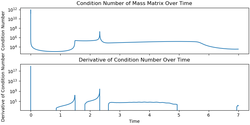
maximal condition number = 9.17e+11
minimal condition number = 9.33e+02
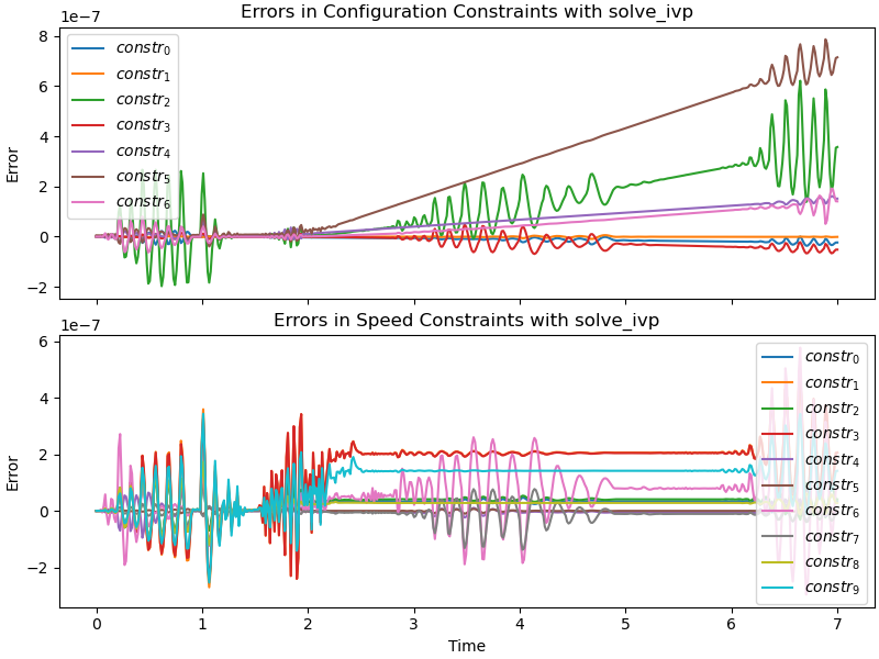
See how well the constraints are kept.
fig, ax = plt.subplots(2, 1, figsize=(8, 6), layout='constrained', sharex=True)
for i in range(7):
ax[0].plot(resultat1.t, config_constr_lam(*resultat1.y, *args)[i].T,
label=f'$constr_{i}$')
ax[0].set_ylabel('Error')
ax[1].set_ylabel('Error')
ax[1].set_xlabel('Time')
ax[0].set_title('Errors in Configuration Constraints with solve_ivp')
ax[1].set_title('Errors in Speed Constraints with solve_ivp')
ax[0].legend()
for i in range(10):
ax[1].plot(resultat1.t, speed_constr_lam(*resultat1.y, *args)[i].T,
label=f'$constr_{i}$')
_ = ax[1].legend()
Plot some coordinates.
Note the almost non-differentiable changes in some generalized coordinate at some points in time. (in the plot at around 1.5 sec)
bezeichnung = [str(i) for i in q_ind + q_dep + u_ind + u_dep]
fig, ax = plt.subplots(2, 1, figsize=(8, 6.5), constrained_layout=True,
sharex=True)
for i in range(12, 24):
ax[0].plot(sys_times[0: resultat.shape[0]], resultat[:, i],
label=bezeichnung[i])
ax[0].set_title('Generalized speeds')
ax[0].legend(loc='upper right')
for i in range(0, 12):
ax[1].plot(sys_times[0: resultat.shape[0]], resultat[:, i],
label=bezeichnung[i])
ax[1].set_title('Generalized coordinates')
ax[1].set_xlabel('Time [s]')
_ = ax[1].legend(loc='upper right')
Plot the energy of the system and a few other quantities of interest.
delta_CPL_z = CPL.pos_from(O).dot(N.z) - gesamt(xL, yL, amplitude, frequenz,
rumpel)
delta_CPL_z = me.msubs(delta_CPL_z, kin_dict)
delta_CPL_z_lam = sm.lambdify(q_ind + q_dep + u_ind + u_dep + pL, delta_CPL_z,
cse=True)
delta_CPR_z = CPR.pos_from(O).dot(N.z) - gesamt(xR, yR, amplitude, frequenz,
rumpel)
delta_CPR_z = me.msubs(delta_CPR_z, kin_dict)
delta_CPR_z_lam = sm.lambdify(q_ind + q_dep + u_ind + u_dep + pL, delta_CPR_z,
cse=True)
kin_energy = sum([body.kinetic_energy(N)
for body in BODY])
kin_energy = me.msubs(kin_energy, kin_dict, all_zero)
Dmc_dist = DmcL.pos_from(DmcR).magnitude()
Dmc_dist = me.msubs(Dmc_dist, kin_dict)
Dmc_dist_lam = sm.lambdify(q_ind + q_dep + u_ind + u_dep + pL, Dmc_dist,
cse=True)
pot_energy = sum([body.masscenter.pos_from(O).dot(N.z) * body.mass * g
for body in BODY])
pot_energy = me.msubs(pot_energy, kin_dict)
kin_lam = sm.lambdify(q_ind + q_dep + u_ind + u_dep + pL, kin_energy, cse=True)
pot_lam = sm.lambdify(q_ind + q_dep + u_ind + u_dep + pL, pot_energy, cse=True)
kin_np = np.empty(resultat.shape[0])
pot_np = np.empty(resultat.shape[0])
total_np = np.empty(resultat.shape[0])
dist_np = np.empty(resultat.shape[0])
CPL_z_np = np.empty(resultat.shape[0])
CPR_z_np = np.empty(resultat.shape[0])
for i in range(resultat.shape[0]):
kin_np[i] = kin_lam(*resultat[i], *pL_vals)
pot_np[i] = pot_lam(*resultat[i], *pL_vals)
total_np[i] = kin_np[i] + pot_np[i]
dist_np[i] = Dmc_dist_lam(*resultat[i], *pL_vals)
CPL_z_np[i] = delta_CPL_z_lam(*[resultat[i, j] for j in range(24)],
*pL_vals)
CPR_z_np[i] = delta_CPR_z_lam(*[resultat[i, j] for j in range(24)],
*pL_vals)
fig, ax = plt.subplots(2, 1, figsize=(8, 4), constrained_layout=True)
ax[0].plot(sys_times[0: resultat.shape[0]], kin_np, label='kinetic energy')
ax[0].plot(sys_times[0: resultat.shape[0]], pot_np, label='potential energy')
ax[0].plot(sys_times[0: resultat.shape[0]], total_np, label='total energy')
ax[0].legend(loc='upper left')
ax[1].plot(sys_times[0: resultat.shape[0]], dist_np,
label='distance between centers of mass')
ax[1].plot(sys_times[0: resultat.shape[0]], CPL_z_np,
label='CPL z coordinate')
ax[1].plot(sys_times[0: resultat.shape[0]], CPR_z_np,
label='CPR z coordinate')
ax[1].legend(loc='upper left')
ax[0].set_title('Energy of the system')
ax[1].set_title('Distance between centers of mass and '
'z coordinates of CPL and CPR')
ax[1].set_xlabel('Time [s]')
ax[0].set_ylabel('Energy [J]')
ax[1].set_ylabel('Distance [m]')
max_dist = np.max(dist_np)
min_dist = np.min(dist_np)
print("Error in distance between centers of mass from being constant: "
f"{(max_dist - min_dist) / min_dist:.4e}")
if reibung1 == 0.0:
print("Error in the total energy from being constant: "
f"{(np.max(total_np) - np.min(total_np)) / np.max(total_np):.4e}")
print(F"error in CPL z coordinate from being equal to the road height: "
f"{(np.max(CPL_z_np) - np.min(CPL_z_np)):.4e}")
print(F"error in CPR z coordinate from being equal to the road height: "
f"{(np.max(CPR_z_np) - np.min(CPR_z_np)):.4e}")
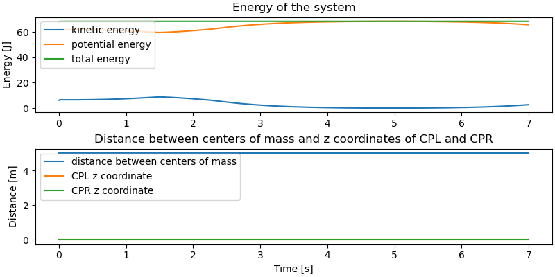
Error in distance between centers of mass from being constant: 0.0000e+00
Error in the total energy from being constant: 7.1880e-03
error in CPL z coordinate from being equal to the road height: 0.0000e+00
error in CPR z coordinate from being equal to the road height: 2.0622e-07
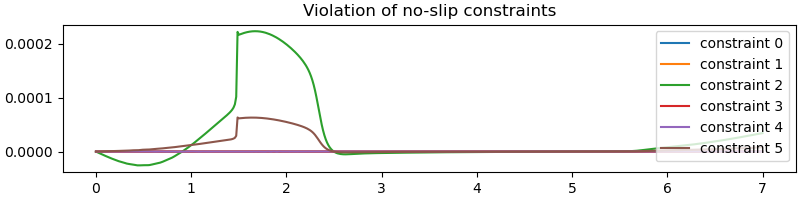
How well are the no slip conditions in Z direction kept? Note: they are not part of the constraints, but result from the fact that the wheels must stay on the surface.
constr_no_slip_test = sm.Matrix([
deltaL_vel.dot(frame.x),
deltaL_vel.dot(frame.y),
deltaL_vel.dot(frame.z),
deltaR_vel.dot(frame.x),
deltaR_vel.dot(frame.y),
deltaR_vel.dot(frame.z),
]).subs(kin_dict)
constr_no_slip_test = me.msubs(constr_no_slip_test, all_zero)
constr_no_slip_test = [constr_no_slip_test[i]
for i in range(constr_no_slip_test.shape[0])]
constr_no_slip_test_lam = sm.lambdify(q_ind + q_dep + u_ind + u_dep +
pL, constr_no_slip_test, cse=True)
constr_no_slip_test_np = np.empty((resultat.shape[0], 6))
for i in range(resultat.shape[0]):
constr_no_slip_test_np[i] = constr_no_slip_test_lam(*resultat[i], *pL_vals)
fig, ax = plt.subplots(1, 1, figsize=(8, 2), constrained_layout=True)
for i in (2, 5):
ax.plot(sys_times[0: resultat.shape[0]], constr_no_slip_test_np[:, i],
label=f'constraint {i}')
ax.legend(loc='upper right')
_ = ax.set_title('Violation of no-slip constraints')
Plot the reaction forces. The log scale is used to see the jump in values better. As the reaction forces are both positive and negative, the absolute value is plotted.
The sum should be nearly zero, maybe the difference is due to numerical errors.
RHS = np.empty((resultat.shape[0], 24))
for i in range(resultat.shape[0]):
RHS[i, :] = np.linalg.solve(MM_lam(*resultat[i, :], *args),
force_lam(*resultat[i, :], *args)).squeeze()
Lfx_np = np.empty(resultat.shape[0])
Lfy_np = np.empty(resultat.shape[0])
Lfz_np = np.empty(resultat.shape[0])
Rfx_np = np.empty(resultat.shape[0])
Rfy_np = np.empty(resultat.shape[0])
Rfz_np = np.empty(resultat.shape[0])
for i in range(resultat.shape[0]):
AR_value = AR_lam(*RHS[i, 12: 24], *resultat[i, :], *pL_vals)
bR_value = bR_lam(*RHS[i, 12: 24], *resultat[i, :], *pL_vals)
solution = np.linalg.solve(AR_value, bR_value).squeeze()
Lfx_np[i], Lfy_np[i], Lfz_np[i], Rfx_np[i], Rfy_np[i], Rfz_np[i] = \
solution
fig, ax = plt.subplots(3, 1, figsize=(8, 10), constrained_layout=True)
ax[0].plot(resultat1.t, np.abs(Lfx_np), label='Lfx')
ax[0].plot(resultat1.t, np.abs(Lfy_np), label='Lfy')
ax[0].plot(resultat1.t, np.abs(Lfz_np), label='Lfz')
ax[0].set_yscale('log')
ax[0].set_xlabel('Time')
ax[0].set_ylabel('[N]')
ax[0].set_title('|Reaction Forces| over time, left wheel')
ax[0].legend()
ax[1].plot(resultat1.t, np.abs(Rfx_np), label='Rfx')
ax[1].plot(resultat1.t, np.abs(Rfy_np), label='Rfy')
ax[1].plot(resultat1.t, np.abs(Rfz_np), label='Rfz')
ax[1].set_xlabel('Time')
ax[1].set_yscale('log')
ax[1].set_ylabel('[N]')
ax[1].set_title('|Reaction Forces| over time, right wheel')
ax[1].legend()
deltax = Lfx_np + Rfx_np
deltay = Lfy_np + Rfy_np
deltaz = Lfz_np + Rfz_np
ax[2].plot(resultat1.t, np.abs(Lfx_np + Rfx_np), label='deltax')
ax[2].plot(resultat1.t, np.abs(Lfy_np + Rfy_np), label='deltay')
ax[2].plot(resultat1.t, np.abs(Lfz_np + Rfz_np), label='deltaz')
ax[2].set_yscale('log')
ax[2].set_ylabel('[N]')
ax[2].set_title('Reaction Forces over time, sum of left and right wheels')
ax[2].legend()
_ = ax[2].set_xlabel('Time')
Animation
fps = 20
t_arr = resultat1.t
state_sol = interp1d(t_arr, resultat1.y.T, kind='cubic', axis=0)
coordinates = DmcL.pos_from(O).to_matrix(N)
for point in (DmcR, m_DmcL, m_DmcR):
coordinates = coordinates.row_join(point.pos_from(O).to_matrix(N))
coords_lam = sm.lambdify(qL + pL, coordinates, cse=True)
max_x = np.max(np.concatenate((resultat1.y.T[:, 0], resultat1.y.T[:, 6])))
max_y = np.max(np.concatenate((resultat1.y.T[:, 1], resultat1.y.T[:, 7])))
min_x = np.min(np.concatenate((resultat1.y.T[:, 0], resultat1.y.T[:, 6])))
min_y = np.min(np.concatenate((resultat1.y.T[:, 1], resultat1.y.T[:, 7])))
gesamt_plot_lam = sm.lambdify([x_h, y_h, amplitude, frequenz],
gesamt_plot(x_h, y_h, amplitude, frequenz),
cse=True)
max_radius = 2.0 * max(rL1, rR1)
xx = np.linspace(min_x-max_radius, max_x+max_radius, 100)
yy = np.linspace(min_y-max_radius, max_y+max_radius, 100)
XX, YY = np.meshgrid(xx, yy)
ZZ = gesamt_plot_lam(XX, YY, amplitude1, frequenz1)
fig, ax = plt.subplots(figsize=(7, 7))
ax.set_xlim(min_x-max_radius, max_x+max_radius)
ax.set_ylim(min_y-max_radius, max_y+max_radius)
ax.set_aspect('equal')
ax.set_xlabel('x', fontsize=15)
ax.set_ylabel('y', fontsize=15)
cf = ax.contourf(XX, YY, ZZ, levels=50, cmap='viridis')
fig.colorbar(cf, label='z value [m]', shrink=0.8)
line1, = ax.plot([], [], lw=1, marker='o', markersize=0, color='red')
line4 = ax.scatter([], [], color='black', s=20)
line5 = ax.scatter([], [], color='black', s=20)
# ellipses defined in local frame AX
winkel_q2 = state_sol(0)[5]
ellipseL = Ellipse((0, 0), width=2.0*rL1*np.sin(winkel_q2),
height=2.0*rL1,
fill=True, lw=2, color='red', alpha=0.5)
ax.add_patch(ellipseL)
ellipseR = Ellipse((0, 0), width=2.0*rR1*np.sin(winkel_q2),
height=2.0*rR1,
fill=True, lw=2, color='magenta', alpha=0.5)
ax.add_patch(ellipseR)
def update(t):
message = (f'running time {t:.2f} sec \n'
f'the left wheel is red with radius {rL1}, the '
f'right wheel is magenta \n with radius {rR1},'
f' The black dots are the particles attached \n to the wheels')
ax.set_title(message, fontsize=11)
coords = coords_lam(*state_sol(t), *pL_vals)
line1.set_data([coords[0, 0], coords[0, 1]], [coords[1, 0], coords[1, 1]])
line4.set_offsets([coords[0, 2], coords[1, 2]])
line5.set_offsets([coords[0, 3], coords[1, 3]])
# transform from AX → inertial frame
theta = state_sol(t)[4]
X = coords[0, 0]
Y = coords[1, 0]
transform = Affine2D().rotate(theta).translate(X, Y) + ax.transData
ellipseL.set_width(2.0*rL1*np.sin(state_sol(t)[5]))
ellipseL.set_transform(transform)
X = coords[0, 1]
Y = coords[1, 1]
transform = Affine2D().rotate(theta).translate(X, Y) + ax.transData
ellipseR.set_width(2.0*rR1*np.sin(state_sol(t)[5]))
ellipseR.set_transform(transform)
return line1, line4, line5, ellipseL, ellipseR
# Create the animation
animation = FuncAnimation(fig, update,
frames=np.concatenate([np.arange(
0, resultat1.t[-1], 1.0/fps),
[resultat1.t[-1]]]),
interval=1000/fps, blit=False)
plt.show()