Underwater Vehicle (betts-10-6)

This is example 10.6 from Betts’ book “Practical Methods for Optimal Control Using NonlinearProgramming”, 3rd edition, Chapter 10: Test Problems.

Betts gives this as the reference for the problem:

C. Büskens and H. Maurer, SQP-methods for solving optimal control problems with control and state constraints: Adjoint variables, sensitivity analysis and real time control Journal of Computational and Applied Mathematics, 120 (2000), pp. 85-108.

States

• \(y_1, ..., y_{10}\) : state variables

Specifieds

• \(u_1, ..., u_4\) : control variables

import numpy as np
import sympy as sm
import sympy.physics.mechanics as me
import time
from opty import Problem
from opty.utils import create_objective_function, MathJaxRepr

Equations of motion.

t = me.dynamicsymbols._t
y1, y2, y3, y4, y5, y6, y7, y8, y9, y10 = \
    me.dynamicsymbols('y1 y2 y3 y4 y5 y6 y7 y8 y9 y10')
u1, u2, u3, u4 = me.dynamicsymbols('u1 u2 u3 u4')

cx, rx, ux, cz, uz = sm.symbols('cx rx ux cz uz')

uy1 = y1.diff(t)
uy2 = y2.diff(t)
uy3 = y3.diff(t)
uy4 = y4.diff(t)
uy5 = y5.diff(t)
uy6 = y6.diff(t)
uy7 = y7.diff(t)
uy8 = y8.diff(t)
uy9 = y9.diff(t)
uy10 = y10.diff(t)

E = sm.exp(-((y1 - cx)/rx)**2)
Rx = -ux*E*(y1-cx)*((y3 - cz)/cz)**2
Rz = -uz*E*((y3-cz)/cz)**2

eom = sm.Matrix([
    -uy1 + y7*sm.cos(y6)*sm.cos(y5) + Rx,
    -uy2 + y7*sm.sin(y6)*sm.cos(y5),
    -uy3 - y7*sm.sin(y5) + Rz,
    -uy4 + y8 + y9*sm.sin(y4)*sm.tan(y5) + y10*sm.cos(y4)*sm.tan(y5),
    -uy5 + y9*sm.cos(y4) - y10*sm.sin(y4),
    -uy6 + y9*sm.sin(y4)/sm.cos(y5) + y10*sm.cos(y4)/sm.cos(y5),
    -uy7 + u1,
    -uy8 + u2,
    -uy9 + u3,
    -uy10 + u4,
])

MathJaxRepr(eom)

$$\left[\begin{matrix}y_{7} \cos{\left(y_{5} \right)} \cos{\left(y_{6} \right)} - \dot{y}_{1} - \frac{ux \left(- cx + y_{1}\right) \left(- cz + y_{3}\right)^{2} e^{- \frac{\left(- cx + y_{1}\right)^{2}}{rx^{2}}}}{cz^{2}}\\y_{7} \sin{\left(y_{6} \right)} \cos{\left(y_{5} \right)} - \dot{y}_{2}\\- y_{7} \sin{\left(y_{5} \right)} - \dot{y}_{3} - \frac{uz \left(- cz + y_{3}\right)^{2} e^{- \frac{\left(- cx + y_{1}\right)^{2}}{rx^{2}}}}{cz^{2}}\\y_{10} \cos{\left(y_{4} \right)} \tan{\left(y_{5} \right)} + y_{8} + y_{9} \sin{\left(y_{4} \right)} \tan{\left(y_{5} \right)} - \dot{y}_{4}\\- y_{10} \sin{\left(y_{4} \right)} + y_{9} \cos{\left(y_{4} \right)} - \dot{y}_{5}\\\frac{y_{10} \cos{\left(y_{4} \right)}}{\cos{\left(y_{5} \right)}} + \frac{y_{9} \sin{\left(y_{4} \right)}}{\cos{\left(y_{5} \right)}} - \dot{y}_{6}\\u_{1} - \dot{y}_{7}\\u_{2} - \dot{y}_{8}\\u_{3} - \dot{y}_{9}\\u_{4} - \dot{y}_{10}\end{matrix}\right]$$

Set Up the Optimization Problem and Solve it

t0, tf = 0.0, 1.0
num_nodes = 51
interval_value = (tf - t0)/(num_nodes - 1)

state_symbols = (y1, y2, y3, y4, y5, y6, y7, y8, y9, y10)
specified_symbols = (u1, u2, u3, u4)

Specify the objective function and form the gradient.

obj_func = sm.Integral(u1**2 + u2**2 + u3**2 + u4**2, t)

obj, obj_grad = create_objective_function(
    obj_func,
    state_symbols,
    specified_symbols,
    tuple(),
    num_nodes,
    node_time_interval=interval_value,
)

Specify the symbolic instance constraints, the bounds and the known parameter values.

instance_constraints = (
    y1.func(t0),
    y2.func(t0),
    y3.func(t0) - 0.2,
    y4.func(t0) - np.pi/2,
    y5.func(t0) - 0.1,
    y6.func(t0) + np.pi/4,
    y7.func(t0) - 1.0,
    y8.func(t0),
    y9.func(t0) - 0.5,
    y10.func(t0) - 0.1,
    y1.func(tf) - 1.0,
    y2.func(tf) - 0.5,
    y3.func(tf),
    y4.func(tf) - np.pi/2,
    y5.func(tf),
    y6.func(tf),
    y7.func(tf),
    y8.func(tf),
    y9.func(tf),
    y10.func(tf),
)

bounds = {
    u1: (-15.0, 15.1),
    u2: (-15.0, 15.0),
    u3: (-15.0, 15.0),
    u4: (-15.0, 15.0),
    y4: (np.pi/2 - 0.02, np.pi/2 + 0.02),
}

par_map = {
    cx: 0.5,
    rx: 0.1,
    ux: 2.0,
    cz: 0.1,
    uz: 0.1,
}

Create the Problem instance.

prob = Problem(
    obj,
    obj_grad,
    eom,
    state_symbols,
    num_nodes,
    interval_value,
    instance_constraints=instance_constraints,
    known_parameter_map=par_map,
    bounds=bounds,
    time_symbol=t
)

Give some rough estimates for the trajectories.

initial_guess = np.zeros(prob.num_free)

Find the optimal solution.

start = time.time()
solution, info = prob.solve(initial_guess)
end = time.time()
print(info['status_msg'])
Jstar = 236.527851
print(f"Objective value achieved: {info['obj_val']:.4f}, as per the book " +
      f"it is {Jstar:.4f}, so the error is: "
      f"{(info['obj_val'] - Jstar)/Jstar*100:.3f} % ")
print(f"Time taken to solve the optimization problem : {end - start:.2f} s")

b'Algorithm terminated successfully at a locally optimal point, satisfying the convergence tolerances (can be specified by options).'
Objective value achieved: 236.7522, as per the book it is 236.5279, so the error is: 0.095 %
Time taken to solve the optimization problem : 2.93 s

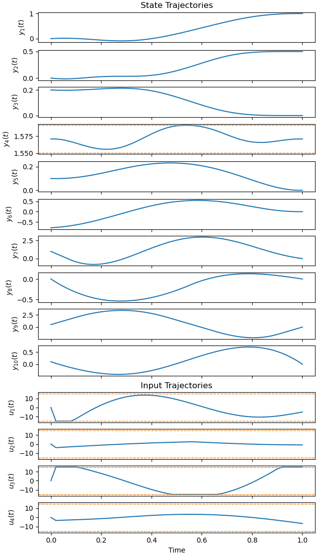
Plot the optimal state and input trajectories.

_ = prob.plot_trajectories(solution, show_bounds=True)

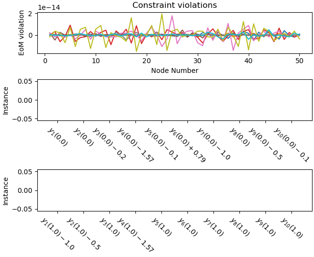
Plot the constraint violations.

_ = prob.plot_constraint_violations(solution)

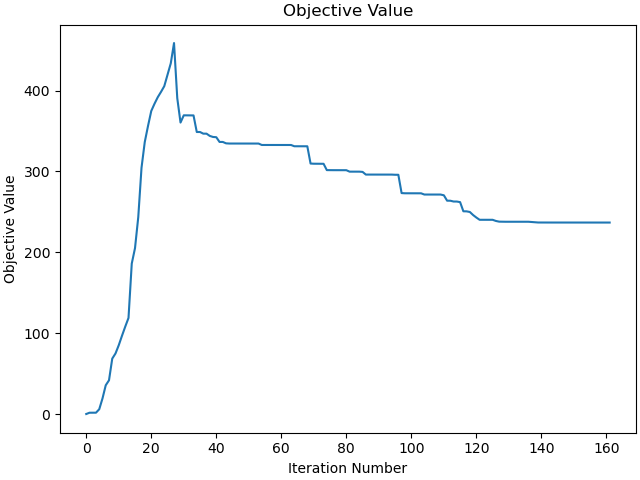
Plot the objective function as a function of optimizer iteration.

_ = prob.plot_objective_value()