Note
Go to the end to download the full example code.
Disc on Very Uneven Street, No Jumping Allowed
Objectives
Show how to use the events keyword of scipy.integrate.solve_ivp to interrupt the numerical integration, when some event occurs. (Here: when a second contact point between street and disc is about to happen.)
Show that the reaction forces may appear in the force vector of Kane’s equations, and how to eliminate then: just set them to zero.
Description
A homogeneous disc with radius r and mass m is running on an uneven ‘street’ without sliding. The disc is not allowed to jump, hence one can calculate the reaction forces needed to hold it on the street at all times.
The ‘overall’ shape of the street is modelled as a parabola (called strassen_form), the unevenness is modelled as a sum of sin functions (called strasse) with each term having a smaller amplitude and higher frequency as the previous one. the ‘street itself’ is the sum of strasse and strassen_form, called gesamt.
When \(r < | \dfrac{(1 + \left(\frac{d}{dx}(gesamt(x(t)))\right)^{3/2}} {\frac{d^2}{dx^2}\left(gesamt(x(t))\right)}|\), the disc will always have only one contact point. If this inequality does not hold, there may be a second contact point. (The formula for osculating radius (Krümmungsradius) is from Wikipedia.) The disc is supposed to run over these ‘pot holes’. The key word events is used in solve_ivp to get the event: a second contact point is there.
Note
When a new contact point is found, the total energy must remain constant, but the moment of inertia will in general be different. So \(\frac{d}{dt}q(t)\) will in general change discontinuously.
Variables
\(q_1, u_1\): rotation of the disc and its speed
\(x, u_x\): loction of the contact point and the speed of successive contact points
N: inertial frame
\(P_0\) point fixed in N
\(A_2\) body fixed frame of disc
\(Dmc\): center of disc
\(Dmc_o\): location of observer
\(CP\): contact point between disc and street
\(m\): mass of the disc
\(m_o\): mass of the observer
\(i_{ZZ}\): moment of inertia of the disc aroud the Z axis
\(\alpha, \beta\): location of the observer relative to the center of the disc
\(\textrm{amplitude, frequenz}\): parameters of the street
\(\textrm{reibung}\): friction
\(rhs_1\): just a place holder for \(MM^{-1}\cdot force\) to be calculated later numerically. Needed for the rection force at CP
import sympy as sm
import sympy.physics.mechanics as me
import numpy as np
import matplotlib.pyplot as plt
import time
from scipy.integrate import solve_ivp
from scipy.optimize import fsolve, minimize, root
from matplotlib import animation
from matplotlib import patches
Needed to exit the loop in the function event when a second contact point was found.
class Rausspringen(Exception):
pass
\(q1\) is the angle of the disc, \(u1\) its angular velocity, x is the horizontal position of contact point CP.
q1, x = me.dynamicsymbols('q1 x')
u1, ux = me.dynamicsymbols('u1 ux')
t = me.dynamicsymbols._t
for the reaction forces at the center of mass Dmc.
auxx, auxy, fx, fy = me.dynamicsymbols('auxx auxy fx fy')
A placeholder for \(\dot{u}_1\) in the reaction forces.
rhs1 = me.dynamicsymbols('rhs1')
Parameters of the system. reibung = friction in German.
m, mo, g, r, iZZ, alpha, beta = sm.symbols('m, mo, g, r, iZZ, alpha, beta')
amplitude, frequenz, reibung = sm.symbols('amplitude frequenz reibung')
N = me.ReferenceFrame('N') # fixed inertial frame
A2 = me.ReferenceFrame('A2') # fixed to the disc
P0, CP, Dmc, Dmco = sm.symbols('P0, CP, Dmc, Dmco', cls=me.Point)
Determine the street and its osculating radius (Schmiegekreis).
rumpel = 4 # the higher the number the more 'uneven the street'
def gesamt1(x, amplitude, frequenz):
strasse = sum([amplitude/j * sm.sin(j*frequenz * x)
for j in range(1, rumpel)])
strassen_form = (frequenz/4. * x)**2
return strassen_form + strasse
gesamt = gesamt1(x, amplitude, frequenz)
r_max = (sm.S(1.) + (gesamt.diff(x))**2)**sm.S(3/2)/gesamt.diff(x, 2)
Relationship of x(t) to q(t):
Obviously, \(x(t) = \textrm{function}(q(t), \textrm{gesamt}(x(t), r)\). When the disc is rotated through an angle \(q\), the arc length is \(r\cdot q(t)\).
The arc length of a function f(k(t)) from 0 to \(x(t)\) is \(\int_{0}^{x(t)} \sqrt{1 + \left(\frac{d}{dk}(f(k(t)\right)^2} \,dk\)
This gives the sought after relationship between \(q(t)\) and \(x(t)\):
\(r \cdot (-q(t)) = \int_{0}^{x(t)} \sqrt{1 + \left( \frac{d}{dk} (gesamt(k(t) \right)^2} \,dk\), differentiated w.r.t t:
\(r \cdot (-u) = \sqrt{1 + \left( \frac{d}{dx}(gesamt(x(t)) \right)^2} \cdot \frac{d}{dt}(x(t)\), that is solved for \(\frac{d}{dt} \left(x(t)\right)\):
\(\frac{d}{dt}(x(t)) = \dfrac{-(r \cdot u)} {\sqrt{1 + \left(\frac{d}{dx}(gesamt(x(t)\right)^2}}\)
The - sign is a consequence of the ‘right hand rule’ for frames. This is the sought after first order differential equation for \(x(t)\).
rhs3 = (-u1 * r / sm.sqrt(1. + (gesamt1(x, amplitude, frequenz).diff(x))**2))
The vector perpendicular to the strasse is \(-(\frac{d}{dx}\textrm{gesamt}(x), - 1)\). The leading minus sign, because directed ‘inward’. It points from the contact point CP to the geometric center of the disc Dmc.
The center of the wheel is at distance r from CP, perpendicular to the surface of the street.
vector = (-(gesamt1(x, amplitude, frequenz).diff(x)*N.x - N.y)).simplify()
A2.orient_axis(N, q1, N.z)
A2.set_ang_vel(N, u1 * N.z)
Location of contact point.
CP.set_pos(P0, x*N.x + gesamt1(x, amplitude, frequenz)*N.y)
Location of the center of gravity of the disc.
Dmc.set_pos(CP, r * (vector.normalize()).simplify())
Velocity of CP and Dmc.
One might think, that since CP is momentarily at rest w.r.t. N,
v2pt_theory might work for the speed of Dmc. It does not, as CP does
have a non-zero speed.
Auxuliary speeds auxx and auxy are needed to get the correct reaction
forces at Dmc.
CP.set_vel(N, (CP.pos_from(P0).diff(t, N)).subs({sm.Derivative(x, t): rhs3}))
Dmc.set_vel(N, Dmc.pos_from(P0).diff(t, N).subs({sm.Derivative(x, t): rhs3}) +
auxx*N.x + auxy*N.y)
Set the particle Dmco on the disc.
Dmco.set_pos(Dmc, r * (alpha*A2.x + beta*A2.y))
Dmco.set_vel(N, Dmco.pos_from(P0).diff(t, N).
subs({sm.Derivative(x, t): rhs3, sm.Derivative(q1, t): u1}))
Needed for potting later.
Dmco_pos = [me.dot(Dmco.pos_from(P0), uv) for uv in (N.x, N.y)]
Dmc_pos = [me.dot(Dmc.pos_from(P0), uv) for uv in (N.x, N.y)]
CP_pos = [me.dot(CP.pos_from(P0), uv) for uv in (N.x, N.y)]
This simple function is needed later to see, if there is a second contact point, \(CP_2\), at location \((xh, \textrm{gesamt}(xh, \textrm{frequenz}, \textrm{amplitude}, \textrm{rumpel}))\) Only necessary to look into the direction the disc is moving, and only the interval \((x, 2\cdot r]\)
xh = sm.symbols('xh')
CP2 = me.Point('CP2')
CP2.set_pos(P0, xh*N.x + gesamt1(xh, amplitude, frequenz)*N.y)
abstand2 = Dmc.pos_from(CP2).magnitude()
print('abstand2 DS', me.find_dynamicsymbols(abstand2))
print('abstand2 FS', abstand2.free_symbols)
abstand2_lam = sm.lambdify([x, xh, r, amplitude, frequenz], abstand2,
cse=True)
abstand2 DS {x(t)}
abstand2 FS {r, t, amplitude, xh, frequenz}
Define the bodies.
Iert = me.inertia(A2, 0., 0., iZZ)
Body = me.RigidBody('Body', Dmc, A2, m, (Iert, Dmc))
observer = me.Particle('observer', Dmco, mo)
BODY = [Body, observer]
Set the energies.
kin_energie = ((Body.kinetic_energy(N) + observer.kinetic_energy(N)).
subs({auxx: 0., auxy: 0.}))
pot_energie = (m * g * me.dot(Dmc.pos_from(P0), N.y) + mo * g *
me.dot(Dmco.pos_from(P0), N.y))
Kane’s Equations
determine the external forces, here only gravitational forces
get the equation for the reaction forces. They (of course) depend on the accelerations of the masses, hence on \(rhs = MM^{-1} \cdot force\). It is calculated numerically later on.
add the term to calculate the X - position of CP at the bottom of force. Recall there is a differential equation for x(t).
enlarge the mass matrix appropriately
FL = [(Dmc, -m*g*N.y), (Dmco, -mo*g*N.y), (Dmc, fx*N.x + fy*N.y),
(A2, -reibung*u1*A2.z)]
kd = [u1 - q1.diff(t)]
q = [q1]
u = [u1]
aux = [auxx, auxy]
KM = me.KanesMethod(N, q_ind=q, u_ind=u, kd_eqs=kd, u_auxiliary=aux)
fr, frstar = KM.kanes_equations(BODY, FL)
MM = KM.mass_matrix_full
force = KM.forcing_full
Reaction forces.
eingepraegt = (KM.auxiliary_eqs.subs({sm.Derivative(u1, t): rhs1,
sm.Derivative(x, t): rhs3}))
print('eingepraegt DS', me.find_dynamicsymbols(eingepraegt))
print('eingepraegt free symbols', eingepraegt.free_symbols)
print(f'eingepraegt has {sm.count_ops(eingepraegt)} operations', '\n')
eingepraegt DS {rhs1(t), x(t), u1(t), fy(t), fx(t)}
eingepraegt free symbols {r, t, amplitude, m, frequenz, g}
eingepraegt has 6359 operations
Add rhs3 at the bottom of force, to get d/dt(x) = rhs3. This is to numerically integrate \(\dfrac{dx}{dt}\) to get x(t) The reaction forces \(f_x\) and \(f_y\) appear in force. They are set to zero as they do no work.
force = (sm.Matrix.vstack(force, sm.Matrix([rhs3])).
subs({sm.Derivative(x, t): rhs3, fx: 0., fy: 0.}))
print('force DS', me.find_dynamicsymbols(force))
print('force free symbols', force.free_symbols)
print(f'force has {sm.count_ops(force)} operations',
f'{sm.count_ops(sm.cse(force))} after cse', '\n')
force DS {u1(t), x(t), q1(t)}
force free symbols {r, t, amplitude, m, beta, reibung, alpha, frequenz, g, mo}
force has 13698 operations 318 after cse
Enlarge MM properly.
MM = (sm.Matrix.hstack(MM, sm.Matrix([0., 0.])).
subs({sm.Derivative(x, t): rhs3}))
MM = sm.Matrix.vstack(MM, sm.Matrix([0., 0., 1.]).T)
print('MM DS', me.find_dynamicsymbols(MM))
print('MM free symbols', MM.free_symbols)
print(f'MM has {sm.count_ops(MM)} operations, '
f'{sm.count_ops(sm.cse(MM))} after cse \n')
MM DS {x(t), q1(t)}
MM free symbols {r, t, amplitude, m, beta, iZZ, frequenz, mo, alpha}
MM has 1513 operations, 106 after cse
Compilation.
pL = [m, mo, g, r, iZZ, alpha, beta, amplitude, frequenz, reibung]
qL = q + u + [x]
F = [fx, fy]
MM_lam = sm.lambdify(qL + pL, MM, cse=True)
force_lam = sm.lambdify(qL + pL, force, cse=True)
CP_pos_lam = sm.lambdify(qL + pL, CP_pos, cse=True)
Dmc_pos_lam = sm.lambdify(qL + pL, Dmc_pos, cse=True)
Dmco_pos_lam = sm.lambdify(qL + pL, Dmco_pos, cse=True)
Will be solved for the reaction force \(F = \begin{bmatrix} f_x \\ f_y \end{bmatrix}\) numerically later.
eingepraegt_lam = sm.lambdify(F + qL + pL + [rhs1], eingepraegt, cse=False)
This is needed to plot the shape of the street.
strasse_lam = sm.lambdify([x] + pL, gesamt, cse=True)
kin_lam = sm.lambdify(qL + pL, kin_energie, cse=True)
kin1_lam is needed further down for fsolve, where one has to solve for u1.
kin1_lam = sm.lambdify([u1] + [q1, x] + pL, kin_energie, cse=True)
pot_lam = sm.lambdify(qL + pL, pot_energie, cse=True)
r_max_lam = sm.lambdify([x] + pL, r_max, cse=True)
Numerical integration
A: Parameter / initial values
\(q_{11}, u_{11}\): rotation of the disc and its speed
\(x_1, u_{x1}\): location of the contact point and the speed of successive contact points
\(m_1\): mass of the disc
\(m_{o1}\): mass of the observer
\(i_{ZZ1}\): moment of inertia of the disc aroud the Z axis
\(\alpha_1, \beta_1\): location of the observer relative to the center of the disc
\(\textrm{amplitude}_1, \textrm{frequenz}_1\): parameters of the street
\(\textrm{reibung}_1\): friction
While it makes sense to call these values similar to their names when setting up Kane’s equations, avoid the same name: The symbols / dynamic symbols get overwritten, with unintended consequences. In order to find a second contaxct point, at least the way I could come up with, step_size and max_step have to be small, slowing down the integration.
Input parameters
m1 = 1.0
mo1 = 1.0
r1 = 2.
alpha1, beta1 = 0., 0.99
amplitude1 = 1.
frequenz1 = 0.9 # the smaller this number, the more 'even' the street
reibung1 = 0.0 # Friction
intervall = 10.0 # time inverval of integration is [0., intervall]
starting values. As the disc is symmetric \(q_{11}\), it plays no real role
q11 = 0.0
u11 = 3.5 # starting angular velocity of disc.
x1 = 7.5 # Starting X position of disc.
step_size = 0.01 # Stepsize to be used to search for the second CP
max_step = 0.01 # Max. stepsize for solve_ivp
Determine the number of times given out by the solution of solve_ivp
punkte = 500
schritte = int(intervall * punkte)
iZZ1 = 1/2 * m1 * r1**2
pL_vals = [m1, mo1, 9.8, r1, iZZ1, alpha1, beta1, amplitude1, frequenz1,
reibung1]
y0 = [q11, u11, x1]
print('Arguments')
print('[m, mo1, g, r, iZZ, iXY, alpha, beta, amplitude, frequenz, reibung]')
print(pL_vals, '\n')
print('[q11, u11, x1]')
print(y0, '\n')
startwert = y0[2] # just needed for the plots below
startomega = y0[1] # dto.
Arguments
[m, mo1, g, r, iZZ, iXY, alpha, beta, amplitude, frequenz, reibung]
[1.0, 1.0, 9.8, 2.0, 2.0, 0.0, 0.99, 1.0, 0.9, 0.0]
[q11, u11, x1]
[0.0, 3.5, 7.5]
Find the minimal osculating radius along the street
def func(x, args):
# just needed to get the arguments matching for minimize
return np.abs(r_max_lam(x, *args))
x0 = 0.1 # initial guess
minimal = minimize(func, x0, pL_vals)
if pL_vals[3] < (x111 := minimal.get('fun')):
print(f'disc radius = {pL_vals[3]} is less than minimal osculating '
f'radius = {x111:.2f}, hence no 2nd contact point possible. \n')
else:
print(f'disc radius {pL_vals[3]} is larger than minimal osculating '
f'radius {x111:.2f}, hence a second contact point may happen. \n')
disc radius 2.0 is larger than minimal osculating radius 0.27, hence a second contact point may happen.
Check, that at the initial position, no second contact point is nearby. vorzeichen determines, which direction one must look at for a possible CP2
for vorzeichen in (-1., 1.):
bereich = np.linspace(x1 - vorzeichen*step_size, x1 - vorzeichen * 2. *
(r1+1.), int(2.*r1/step_size))
for xh1 in bereich:
if abstand2_lam(x1, xh1, r1, amplitude1, frequenz1) <= r1:
raise Exception('change starting point')
else:
pass
When a new contact point is found, the total energy must remain constant, but the moment of inertia will in general be different. So \(\frac{d}{dt}q(t)\) must in general change discontinuously. This function is used to calculate the new angular velocity \(\frac{d}{dt}q(t)\).
def funcCP(x0, args):
return (
kin1_lam(x0, args[0], args[1], *args[5]) - kin_lam(args[2], args[3],
args[4], *args[5]))
B: Actual numerical integration starts here.
The function event is needed to stop solve_ivp when a second contact point is found, see the documentation of solve_ivp for details. Of course, one only has to look for second contact points in the direction of the movement at the time. Once a second contact point is found, the numerical integration is stopped, and its results stored in ergebnis. Then a new numrical integration is started with new initial conditions. \(CP_{2x}\) is needed for the next integration, but cannot be returned, as solve_ivp needs a defined output of the event function. Hence it is made a global variable.
NOTES: The events keyword of solve_ivp requires a continuous function f(t, y, args) with {event happened at \(t_0, y_0 <=> f(t_0, y_0, args) = 0.0\) In this case, with a numerical criterium, the right way to do it is like this:
a helpful person in Stack Overflow explained it to me:
As long as the event has not occured, the function returns -1. When the event did occur, it returns +1. This works fine.
start1 = time.time()
schritte = int(intervall * punkte)
times = np.linspace(0, intervall, schritte)
CP2x = 0.0
y0 = [q11, u11, x1]
zaehl_event = 0
def event(t, y, args):
global CP2x, zaehl_event
zaehl_event += 1
# determines, which direction we must look at for CP2
vorzeichen = np.sign(y[1])
bereich = np.linspace(y[2] - 5.0 * vorzeichen*step_size, y[2] -
vorzeichen * 3.0 * r1, int(2.0*r1/step_size))
for xh1 in bereich:
try:
if abstand2_lam(y[2], xh1, r1, amplitude1, frequenz1) <= r1:
raise Rausspringen()
else:
pass
except Rausspringen:
# event_info = True shows, how solve_ivp searches for the exact
# location where the even took place
if event_info:
print(
f'second CP, as '
f'{(abstand2_lam(y[2], xh1, r1, amplitude1,
frequenz1) - r1):.3f} '
f'<=0, at time {t:.3f} and location {xh1:.3f}')
CP2x = xh1
return 1. # 0 a second contact point was found
return -1. # 1 no second contact point
If True, this stops the integration if event occurs
event.terminal = True
If True, data related to the occurrence of events are printed
event_info = False
The gradient function for solve_ivp.
def gradient(t, y, args):
vals = np.concatenate((y, args))
sol = np.linalg.solve(MM_lam(*vals), force_lam(*vals))
return np.array(sol).T[0]
runtime = 0.
starttime = 0.
starttime1 = 0.
ergebnis = []
Here the ‘piecewise’ integration starts.
while starttime < intervall:
resultat1 = solve_ivp(gradient, (starttime, float(intervall)), y0,
t_eval=times, args=(pL_vals,), atol=1.e-7,
rtol=1.e-7, max_step=max_step, events=event,
method='Radau')
resultat = resultat1.y.T
if event_info:
print(resultat1.message)
print('resultat shape', resultat.shape)
if resultat1.y_events[0].size > 0.:
height = strasse_lam(resultat1.y_events[0][0][2], *pL_vals)
if event_info:
print('generalized coordinates at exit time, height of CP '
f'{resultat1.y_events[0][0][0]:.3f} '
f'{resultat1.y_events[0][0][1]:.3f} '
f'{resultat1.y_events[0][0][2]:.3f} {height:.3f}')
hilfs0 = resultat1.y_events[0][0][0]
hilfs1 = resultat1.y_events[0][0][1]
hilfs2 = resultat1.y_events[0][0][2]
args1 = [hilfs0, CP2x] + [hilfs0, hilfs1, hilfs2, pL_vals]
x0 = hilfs1
# Force the total energy to be constant.
# Sometimes iterating improves the accuracy
for _ in range(1):
hilfs3 = fsolve(funcCP, x0, args1)
hilfs3 = hilfs3[0]
x0 = hilfs3
y0 = [resultat1.y_events[0][0][0], hilfs3, CP2x]
height = strasse_lam(CP2x, *pL_vals)
if event_info:
print('initial values for the next integration, height of new '
f'CP {hilfs0:.3f} {hilfs3:.3f}' +
f' {CP2x:.3F} {height:.3f}' + '\n')
starttime = resultat1.t_events[0][0]
schritte = int((intervall - starttime) * punkte)
times = np.linspace(starttime, intervall, schritte)
ergebnis.append(resultat)
else:
break
print(f"To numerically integrate an intervall of {intervall} sec "
f"took {time.time() - start1:.5f} sec ")
print(resultat1.message)
To numerically integrate an intervall of 10.0 sec took 8.36674 sec
The solver successfully reached the end of the integration interval.
Stack the individual results of the various integrations, to get the complete results.
resultat = np.vstack(ergebnis)
print(resultat.shape)
(4956, 3)
Set these values for the subsequent plots below.
schritte = resultat.shape[0]
times = np.linspace(0., intervall, schritte)
print('how often did solve_ivp call event:', zaehl_event)
how often did solve_ivp call event: 2830
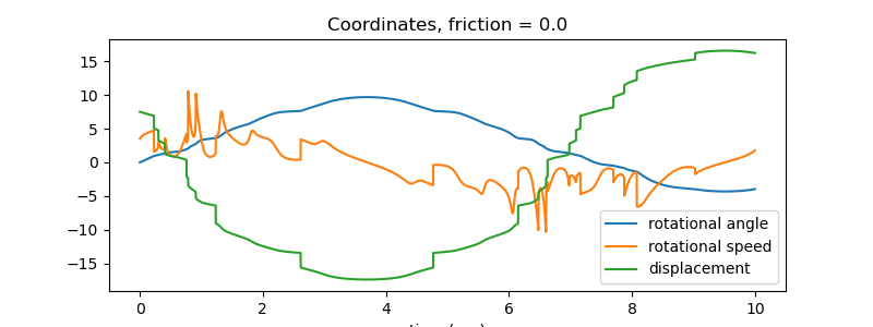
Plot the generalized coordinates and speeds
Dmc_X = np.empty(schritte)
Dmc_Y = np.empty(schritte)
for i in range(schritte):
Dmc_X[i], Dmc_Y[i] = Dmc_pos_lam(*[resultat[i, j]
for j in range(resultat.shape[1])],
*pL_vals)
fig, ax = plt.subplots(figsize=(8, 3))
for i, j in zip(range((resultat.shape[1])), ('rotational angle',
'rotational speed',
'displacement')):
ax.plot(times, resultat[:, i], label=j)
ax.set_title('Coordinates, friction = {}'.format(reibung1))
ax.set_xlabel('time (sec)')
_ = ax.legend()
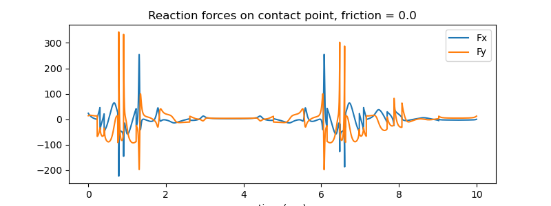
Plot the reaction forces
RHS is calculated numerically, too large to do it symbolically. Needed for the reaction forces.
RHS1 = np.zeros((schritte, resultat.shape[1]))
for i in range(schritte):
RHS1[i, :] = np.linalg.solve(
MM_lam(*[resultat[i, j] for j in range(resultat.shape[1])], *pL_vals),
force_lam(*[resultat[i, j] for j in range(resultat.shape[1])],
*pL_vals)).reshape(resultat.shape[1])
print('RHS1 shape', RHS1.shape)
def func(x11, *args):
return eingepraegt_lam(*x11, *args).reshape(len(F))
kraft = np.empty((schritte, len(F)))
x0 = tuple([1. for i in range(len(F))]) # initial guess
for i in range(schritte):
for _ in range(1):
y00 = [resultat[i, j] for j in range(resultat.shape[1])]
args = tuple((y00 + pL_vals + [RHS1[i, 1]]))
A = root(func, x0, args=args) # numerically find fx, fy
x0 = tuple(A.x) # updated initial guess, should improve convergence
kraft[i] = A.x
fig, ax = plt.subplots(figsize=(8, 3))
ax.plot(times, kraft[:, 0], label='Fx')
ax.plot(times, kraft[:, 1], label='Fy')
ax.set_title(f'Reaction forces on contact point, friction = {reibung1}')
ax.set_xlabel('time (sec)')
_ = ax.legend()
RHS1 shape (4956, 3)
Plot the energies of the system.
kin_np = np.empty(schritte)
pot_np = np.empty(schritte)
total_np = np.empty(schritte)
for i in range(schritte):
kin_np[i] = kin_lam(*[resultat[i, j]
for j in range(resultat.shape[1])], *pL_vals)
pot_np[i] = pot_lam(*[resultat[i, j]
for j in range(resultat.shape[1])], *pL_vals)
total_np[i] = kin_np[i] + pot_np[i]
if pL_vals[-1] == 0.:
print('Max deviation from constant of total energy is {:.2e} '
'% of max total energy'
.format((max(total_np) - min(total_np))/max(total_np) * 100.))
print('Max absolute deviation from constant of total energy is {:.2e} Nm'
.format((np.max(total_np) - np.min(total_np))))
fig, ax = plt. subplots(figsize=(8, 3))
ax.plot(times, kin_np, label='kinetic energy')
ax.plot(times, pot_np, label='pos energy')
ax.plot(times, total_np, label='total energy')
ax.set_title(f'Energy of the disc, friction = {reibung1} '
f'frequenz = {frequenz1}')
ax.set_xlabel('time (sec)')
_ = ax.legend()
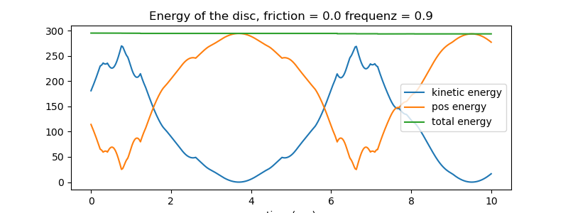
Max deviation from constant of total energy is 6.03e-01 % of max total energy
Max absolute deviation from constant of total energy is 1.78e+00 Nm
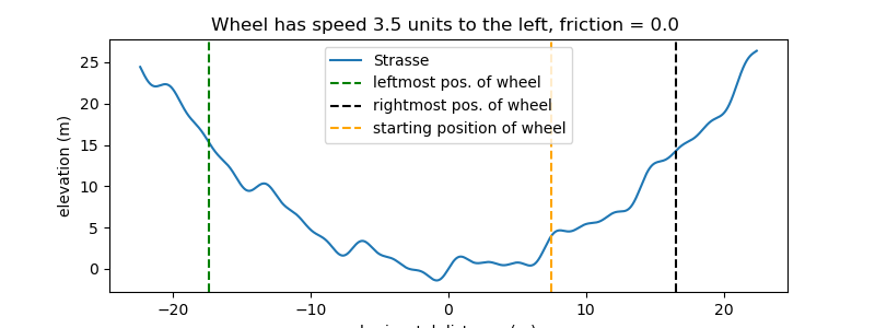
Plot the street and the extreme positions of the disc.
fig, ax = plt.subplots(figsize=(8, 3))
links = np.min(resultat[:, 2])
rechts = np.max(resultat[:, 2])
ruhe = np.mean([resultat[-30::, 2]]) # get approx. rest position of wheel
maximal = max(np.abs(links), np.max(rechts))
times1 = np.linspace(-maximal-5, maximal+5, schritte)
ax.plot(times1, strasse_lam(times1, *pL_vals), label='Strasse')
if pL_vals[-1] != 0.:
ax.axvline(ruhe, ls='--', color='red', label='approx. final pos. '
'of wheel')
ax.axvline(links, ls='--', color='green', label='leftmost pos. of wheel')
ax.axvline(rechts, ls='--', color='black', label='rightmost pos. of wheel')
ax.axvline(startwert, ls='--', color='orange', label='starting position '
'of wheel')
if startomega > 0.:
richtung = 'left'
else:
richtung = 'right'
text = ('Wheel has speed ' + str(np.abs(startomega)) + ' units to the ' +
richtung)
plt.title(text + f', friction = {reibung1} ')
plt.xlabel('horizontal distance (m)')
plt.ylabel('elevation (m)')
_ = ax.legend()
Animation
The blue dot represents the observer. The number of points considered are zeitpunkte. If it builds too slowly, this number may be reduced.
# reduce the number of points of time to around zeitpunkte.
times2 = []
resultat2 = []
index2 = []
zeitpunkte = 100
reduction = max(1, int(len(times)/zeitpunkte))
for i in range(len(times)):
if i % reduction == 0:
times2.append(times[i])
resultat2.append(resultat[i])
schritte2 = len(times2)
print(f'animation used {schritte2} points in time')
resultat2 = np.array(resultat2)
times2 = np.array(times2)
# Location of the center of the disc
Dmcx = np.empty(schritte2)
Dmcy = np.empty(schritte2)
Dmcox = np.empty(schritte2)
Dmcoy = np.empty(schritte2)
for i in range(schritte2):
Dmcx[i], Dmcy[i] = Dmc_pos_lam(*[resultat2[i, j]
for j in range(resultat2.shape[1])],
*pL_vals)
Dmcox[i], Dmcoy[i] = Dmco_pos_lam(*[resultat2[i, j]
for j in range(resultat2.shape[1])],
*pL_vals)
# needed to give the picture the right size.
xmin = min([resultat2[i, 2] for i in range(schritte2)])
xmax = max([resultat2[i, 2] for i in range(schritte2)])
ymin = min([strasse_lam(resultat2[i, 2], *pL_vals) for i in range(schritte2)])
ymax = max([strasse_lam(resultat2[i, 2], *pL_vals) for i in range(schritte2)])
# Data to draw the uneven street
cc = r1
strassex = np.linspace(xmin - 3*cc, xmax + 3.*cc, schritte2)
strassey = [strasse_lam(strassex[i], *pL_vals) for i in range(len(strassex))]
def animate_pendulum(times, x1, y1, x2, y2):
fig, ax = plt.subplots(figsize=(8, 8), subplot_kw={'aspect': 'equal'})
ax.axis('on')
ax.set_xlim(xmin - 3.*cc, xmax + 3.*cc)
ax.set_ylim(ymin - 3.*cc, ymax + 3.*cc)
ax.plot(strassex, strassey)
ax.set_xlabel('horizontal distance (m)')
ax.set_ylabel('elevation (m)')
line1, = ax.plot([], [], 'o-', lw=0.5)
# vertical tracking line
line2 = ax.axvline(resultat2[0, 2], linestyle='--')
# horizontal tracking line
line3 = ax.axhline(
strasse_lam(resultat2[0, 2], *pL_vals), linestyle='--')
# dot on the disc, to show it is rotating
line4, = ax.plot([], [], 'bo', markersize=5)
elli = patches.Circle((x1[0], y1[0]), radius=r1, fill=True, color='red',
ec='black')
ax.add_patch(elli)
def animate(i):
ax.set_title(f'running time {times2[i]:.2f} sec, '
f'friction ={reibung1}', fontsize=15)
elli.set_center((x1[i], y1[i]))
elli.set_height(2.*r1)
elli.set_width(2.*r1)
elli.set_angle(np.rad2deg(resultat[i, 0]))
line1.set_data([x1[i]], [y1[i]]) # center of the disc
line2.set_xdata([resultat2[i, 2]]) # dashed line to mark contact point
line3.set_ydata([strasse_lam(resultat2[i, 2], *pL_vals)]) # dto.
line4.set_data([x2[i]], [y2[i]])
return line1, line2, line3, line4,
anim = animation.FuncAnimation(fig, animate, frames=len(times),
interval=1000*max(times) / len(times),
blit=True)
return anim
anim = animate_pendulum(times2, Dmcx, Dmcy, Dmcox, Dmcoy)
plt.show()
animation used 102 points in time
Total running time of the script: (0 minutes 38.933 seconds)