Note
Go to the end to download the full example code.
Two Body Skateboard
Objectives
Show how to use opty to solve a problem with configuration constraints.
Show how to iterate from a simpler problem, straight lines, to a more complex problem, curved lines.
Description
Admittedly, this is a somewhat contrived example, but it shows how to use opty - and it shows opty’s capabilities to solve what seem to be non-trivial problems.
Two boards are connected by a joint. At the back of the first body and on the front of the second body, there is an axle. The axles can be steered and driven. The goal is to keep the centers of the two bodies on two given lines in the X/Y plane. The two bodies and the axles are modeled as rigid bodies. As gravity plays no role in this model it is disregarded.
Notes
when setting up Kane’s equations of motion, the configuration constraints have to be converted to velocity constraints.
when setting up the equations of motion for opty, either the configuration constraints or the velocity constraints may be added to the equations of motion. Better to use the configuration constraints to avoid the drift inherent in the velocity constraints.
Constants:
\(l\) : length of the bodies [m]
\(m_0, m_b, m_f\) : mass of the bodies, the rear axle, the front axle [kg]
\(iZZ_0, iZZ_b, iZZ_f\) : inertia of the bodies, the rear axle, the front axle [kg m^2]
\(a, b\) : parameters of the streets [m], [1/m]
States:
\(x, y\) : coordinates of the point, where the rear axle attaches to the main body [m]
\(ux, uy\) : their speeds [m/s]
\(q_0, q_1, q_b, q_f\) : gen. coordinates of the main bodies, the rear axle, the front axle [rad]
\(u_0, u_1, u_b, u_f\) : their speeds [rad/s]
Specifieds:
\(T_b, T_f\) : torque at back wheel, torque at front wheel [Nm]
\(F_b, F_f\) : forces on \(A^o_b, A^o_f\) [N]
Further Parameters:
\(N\) : the inertial frame
\(A_0, A_1, A_b, A_f\) : the frames of the bodies
\(O\) : point fixed in the inertial frame
\(P_1\) : the joint between the two bodies
\(A^o_{b}, A^o_{f}\) : the mass centers of the axles
\(A^o_0, A^o_1\) : the mass centers of the bodies
import sympy.physics.mechanics as me
import sympy as sm
import numpy as np
from scipy.optimize import fsolve
from scipy.interpolate import CubicSpline
from opty.direct_collocation import Problem
from opty.utils import create_objective_function
import matplotlib.pyplot as plt
from matplotlib.animation import FuncAnimation
Defines the shape of the two lines to be followed by the centers of the bodies.
def strasse(x, a, b):
return a * (sm.sin(b * x) + sm.cos(3 * b * x))
def strasse1(x, a, b):
return a * sm.sin(b * x) + sm.cos(4 * b * x) + 1.
Kane’s Equations of Motion
N, A0, A1, Ab, Af = sm.symbols('N A0 A1 Ab Af', cls=me.ReferenceFrame)
t = me.dynamicsymbols._t
O, Aob, Ao0, P1, Ao1, Aof = sm.symbols('O Aob Ao0 P1 Ao1 Aof', cls=me.Point)
O.set_vel(N, 0)
q0, q1, qb, qf = me.dynamicsymbols('q_0 q_1 q_b q_f')
u0, u1, ub, uf = me.dynamicsymbols('u_0 u_1 u_b u_f')
x, y = me.dynamicsymbols('x y')
ux, uy = me.dynamicsymbols('u_x u_y')
Tb, Tf, Fb, Ff = me.dynamicsymbols('T_b T_f F_b F_f')
l, m0, mb, mf, iZZ0, iZZb, iZZf = sm.symbols('l m0 mb mf iZZ0, iZZb, iZZf')
a, b = sm.symbols('a b')
A0.orient_axis(N, q0, N.z)
A0.set_ang_vel(N, u0 * N.z)
A1.orient_axis(N, q1, N.z)
A1.set_ang_vel(N, u1 * N.z)
Ab.orient_axis(N, qb, N.z)
Ab.set_ang_vel(N, ub * N.z)
Af.orient_axis(N, qf, N.z)
Af.set_ang_vel(N, uf * N.z)
Aob.set_pos(O, x * N.x + y * N.y)
Aob.set_vel(N, ux * N.x + uy * N.y)
Ao0.set_pos(Aob, l/2 * A0.y)
Ao0.v2pt_theory(Aob, N, A0)
P1.set_pos(Aob, l * A0.y)
P1.v2pt_theory(Aob, N, A0)
Ao1.set_pos(P1, l/2 * A1.y)
Ao1.v2pt_theory(P1, N, A1)
Aof.set_pos(P1, l * A1.y)
Aof.v2pt_theory(P1, N, A1)
constr_Ao0 = (me.dot(Ao0.pos_from(O), N.y) -
strasse(me.dot(Ao0.pos_from(O), N.x), a, b))
constr_Ao0_dt = constr_Ao0.diff(t)
constr_Ao1 = (me.dot(Ao1.pos_from(O), N.y) -
strasse1(me.dot(Ao1.pos_from(O), N.x), a, b))
constr_Ao1_dt = constr_Ao1.diff(t)
I0 = me.inertia(A0, 0, 0, iZZ0)
body0 = me.RigidBody('body0', Ao0, A0, m0, (I0, Ao0))
I1 = me.inertia(A1, 0, 0, iZZ0)
body1 = me.RigidBody('body1', Ao1, A1, m0, (I1, Ao1))
Ib = me.inertia(Ab, 0, 0, iZZb)
bodyb = me.RigidBody('bodyb', Aob, Ab, mb, (Ib, Aob))
If = me.inertia(Af, 0, 0, iZZf)
bodyf = me.RigidBody('bodyf', Aof, Af, mf, (If, Aof))
BODY = [body0, body1, bodyb, bodyf]
FL = [(Aob, Fb * Ab.y), (Aof, Ff * Af.y), (Ab, Tb * N.z), (Af, Tf * N.z)]
kd = sm.Matrix([ux - x.diff(t), uy - y.diff(t), u0 - q0.diff(t),
u1 - q1.diff(t), ub - qb.diff(t), uf - qf.diff(t)])
speed_constr = [constr_Ao0_dt, constr_Ao1_dt]
hol_constr = sm.Matrix([constr_Ao0, constr_Ao1])
q_ind = [x, y, qb, qf]
q_dep = [q0, q1]
u_ind = [ux, uy, ub, uf]
u_dep = [u0, u1]
KM = me.KanesMethod(
N,
q_ind=q_ind,
u_ind=u_ind,
kd_eqs=kd,
q_dependent=q_dep,
u_dependent=u_dep,
configuration_constraints=hol_constr,
velocity_constraints=speed_constr,
)
fr, frstar = KM.kanes_equations(BODY, FL)
eom = kd.col_join(fr + frstar)
eom = eom.col_join(hol_constr)
print(f'eoms contain {sm.count_ops(eom):,} operations and have '
f'shape {eom.shape}')
eoms contain 1,601 operations and have shape (12, 1)
Needed further down for the animation.
strasse2 = strasse(x, a, b)
strasse3 = strasse1(x, a, b)
strasse_lam = sm.lambdify((x, a, b), strasse2, cse=True)
strasse1_lam = sm.lambdify((x, a, b), strasse3, cse=True)
Needed to ensure to configuration constrains are satisfied at the start.
constr_Ao0_lam = sm.lambdify((y, x, q0, a, b, l), constr_Ao0, cse=True)
constr_Ao1_lam = sm.lambdify((q1, x, y, q0, a, b, l), constr_Ao1, cse=True)
Set up the Optimization Problem.
state_symbols = tuple((x, y, q0, q1, qb, qf, ux, uy, u0, u1, ub, uf))
laenge = len(state_symbols)
constant_symbols = (a, b, l, m0, mb, mf, iZZ0, iZZb, iZZf)
specified_symbols = (Fb, Ff, Tb, Tf)
unknown_symbols = []
duration = 7.5
num_nodes = 300
t0, tf = 0.0, duration
interval_value = duration / (num_nodes - 1)
Specify the known system parameters.
par_map = {}
par_map[m0] = 1.0
par_map[mb] = 0.1
par_map[mf] = 0.1
par_map[iZZ0] = 1.0
par_map[iZZb] = 0.1
par_map[iZZf] = 0.1
par_map[l] = 3.0
par_map[a] = 1.75
par_map[b] = 0.0
x1 = 0.0
q01 = -0.5
Calculate the initial value of y, so that the configuration constraint is satisfied. As the initial speeds are set to zero, the resulting speed constraint is satisfied automatically.
def hol_func(x0, *args):
return constr_Ao0_lam(x0, *args)
def hol_func1(x0, *args):
return constr_Ao1_lam(x0, *args)
x0 = 1.0
args = (x1, q01, par_map[a], par_map[b], par_map[l])
y1 = fsolve(hol_func, x0, args)
args = (x1, y1[0], q01, par_map[a], par_map[b], par_map[l])
q11 = fsolve(hol_func1, x0, args)
Set up the objective function.
objective = sm.Integral((Fb**2) + (Ff**2) + (Tb**2) + (Tf**2))
obj, obj_grad = create_objective_function(
objective,
state_symbols,
specified_symbols,
unknown_symbols,
num_nodes,
interval_value,
)
Set up the constraints, and the bounds.
initial_state_constraints = {
x: x1,
y: y1[0],
q0: q01,
q1: q11[0],
qb: -0.2,
qf: -0.3,
ux: 0.0,
uy: 0.0,
u0: 0.0,
u1: 0.0,
ub: 0.0,
uf: 0.0,
}
final_state_constraints = {
x: 12.,
ux: 0.0,
}
instance_constraints = (tuple(xi.subs({t: t0}) - xi_val
for xi, xi_val in
initial_state_constraints.items()) +
tuple(xi.subs({t: tf}) - xi_val
for xi, xi_val in
final_state_constraints.items()))
grenze = 300.0
bounds = {
Fb: (-grenze, grenze),
Ff: (-grenze, grenze),
Tb: (-grenze, grenze),
Tf: (-grenze, grenze),
qb: (-np.pi/2, np.pi/2),
qf: (-np.pi/2, np.pi/2),
}
Solve the Optimization Problem
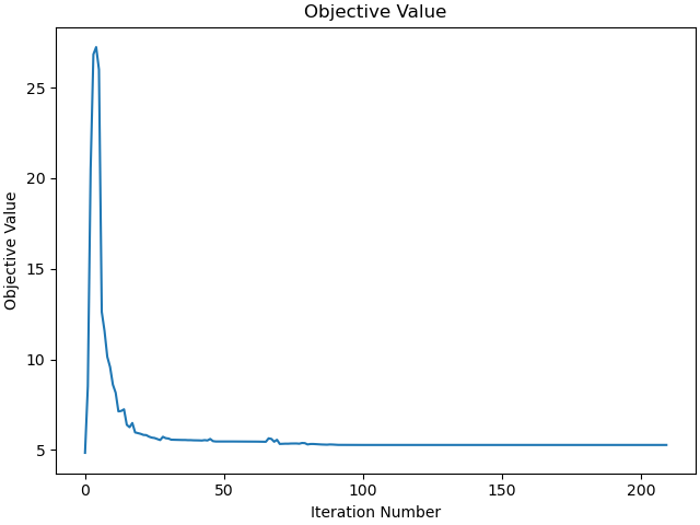
For this problem opty does not find a solution unless either the curves are straight lines or the initial guess is very close to the solution. So the program below iterates from the straight curve to the curve with the desired parameters. Solutions are the initial guess of the next iteration.
inkrement = 0.0125
initial_guess = np.ones((len(state_symbols) +
len(specified_symbols)) * num_nodes) * 0.01
for i in range(15):
par_map[b] = inkrement * i
# As the shape of the curves changes in every loop, the instance
# constraints have to be recalculated to match the configuration
# constraints.
x0 = 1.
args = (x1, q01, par_map[a], par_map[b], par_map[l])
y1 = fsolve(hol_func, x0, args)
args = (x1, y1[0], q01, par_map[a], par_map[b], par_map[l])
q11 = fsolve(hol_func1, x0, args)
initial_state_constraints[y] = y1[0]
initial_state_constraints[q1] = q11[0]
instance_constraints = (tuple(xi.subs({t: t0}) - xi_val
for xi, xi_val in
initial_state_constraints.items()) +
tuple(xi.subs({t: tf}) - xi_val
for xi, xi_val in
final_state_constraints.items()))
# As the instance constraints change, Problem has to be built for every
# iteration.
prob = Problem(
obj,
obj_grad,
eom,
state_symbols,
num_nodes,
interval_value,
known_parameter_map=par_map,
instance_constraints=instance_constraints,
bounds=bounds,
)
prob.add_option('max_iter', 3000)
solution, info = prob.solve(initial_guess)
np.save('skate_solution', solution)
print(f'{i+1} - th iteration')
print('message from optimizer:', info['status_msg'])
print('Iterations needed', len(prob.obj_value))
print(f"objective value {info['obj_val']:.3e} \n")
initial_guess = solution
_ = prob.plot_objective_value()
1 - th iteration
message from optimizer: b'Algorithm terminated successfully at a locally optimal point, satisfying the convergence tolerances (can be specified by options).'
Iterations needed 168
objective value 3.220e+00
2 - th iteration
message from optimizer: b'Algorithm terminated successfully at a locally optimal point, satisfying the convergence tolerances (can be specified by options).'
Iterations needed 93
objective value 3.236e+00
3 - th iteration
message from optimizer: b'Algorithm terminated successfully at a locally optimal point, satisfying the convergence tolerances (can be specified by options).'
Iterations needed 197
objective value 3.130e+00
4 - th iteration
message from optimizer: b'Algorithm terminated successfully at a locally optimal point, satisfying the convergence tolerances (can be specified by options).'
Iterations needed 299
objective value 2.962e+00
5 - th iteration
message from optimizer: b'Algorithm terminated successfully at a locally optimal point, satisfying the convergence tolerances (can be specified by options).'
Iterations needed 109
objective value 3.143e+00
6 - th iteration
message from optimizer: b'Algorithm terminated successfully at a locally optimal point, satisfying the convergence tolerances (can be specified by options).'
Iterations needed 120
objective value 3.482e+00
7 - th iteration
message from optimizer: b'Algorithm terminated successfully at a locally optimal point, satisfying the convergence tolerances (can be specified by options).'
Iterations needed 112
objective value 3.979e+00
8 - th iteration
message from optimizer: b'Algorithm stopped at a point that was converged, not to "desired" tolerances, but to "acceptable" tolerances (see the acceptable-... options).'
Iterations needed 313
objective value 3.932e+00
9 - th iteration
message from optimizer: b'Algorithm terminated successfully at a locally optimal point, satisfying the convergence tolerances (can be specified by options).'
Iterations needed 130
objective value 3.811e+00
10 - th iteration
message from optimizer: b'Algorithm stopped at a point that was converged, not to "desired" tolerances, but to "acceptable" tolerances (see the acceptable-... options).'
Iterations needed 164
objective value 3.942e+00
11 - th iteration
message from optimizer: b'Algorithm terminated successfully at a locally optimal point, satisfying the convergence tolerances (can be specified by options).'
Iterations needed 177
objective value 4.130e+00
12 - th iteration
message from optimizer: b'Algorithm terminated successfully at a locally optimal point, satisfying the convergence tolerances (can be specified by options).'
Iterations needed 219
objective value 4.345e+00
13 - th iteration
message from optimizer: b'Algorithm terminated successfully at a locally optimal point, satisfying the convergence tolerances (can be specified by options).'
Iterations needed 217
objective value 4.587e+00
14 - th iteration
message from optimizer: b'Algorithm terminated successfully at a locally optimal point, satisfying the convergence tolerances (can be specified by options).'
Iterations needed 217
objective value 4.842e+00
15 - th iteration
message from optimizer: b'Algorithm terminated successfully at a locally optimal point, satisfying the convergence tolerances (can be specified by options).'
Iterations needed 210
objective value 5.276e+00
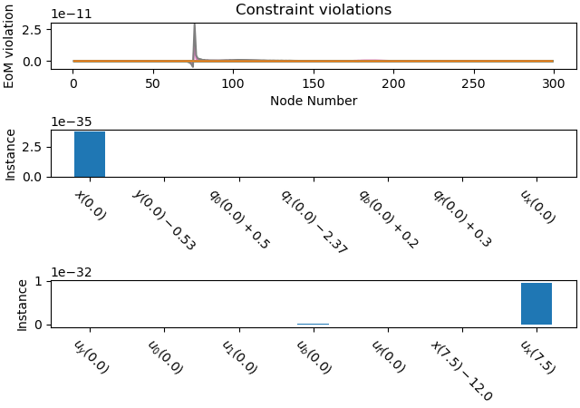
Plot the constraint violations.
_ = prob.plot_constraint_violations(solution)
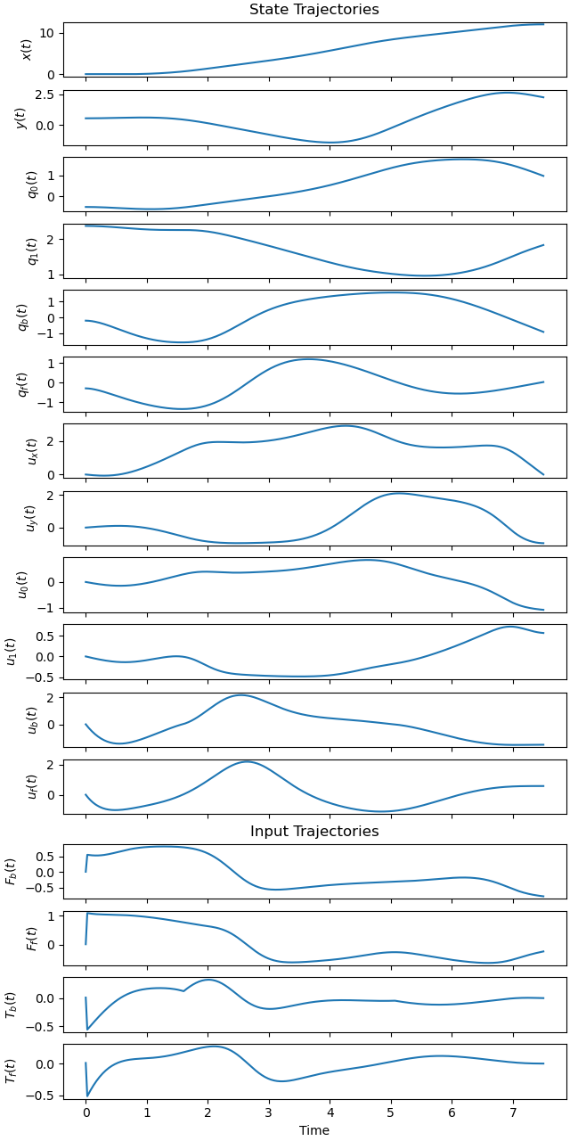
Plot the results.
_ = prob.plot_trajectories(solution)
Animate the Simulation.
fps = 10
state_vals, input_vals, _ = prob.parse_free(solution)
t_arr = np.linspace(t0, tf, num_nodes)
state_sol = CubicSpline(t_arr, state_vals.T)
input_sol = CubicSpline(t_arr, input_vals.T)
# create additional points for the axles
Aobl, Aobr, Aofl, Aofr = sm.symbols('Aobl Aobr Aofl Aofr', cls=me.Point)
Fbq, Ffq = sm.symbols('Fbq Ffq', cls=me.Point)
la = sm.symbols('la')
fb, ff = sm.symbols('f_b f_f')
Aobl.set_pos(Aob, -la/2 * Ab.x)
Aobr.set_pos(Aob, la/2 * Ab.x)
Aofl.set_pos(Aof, -la/2 * Af.x)
Aofr.set_pos(Aof, la/2 * Af.x)
Fbq.set_pos(Aob, fb * Ab.y)
Ffq.set_pos(Aof, ff * Af.y)
coordinates = Aob.pos_from(O).to_matrix(N)
for point in (Ao0, P1, Ao1, Aof, Aobl, Aobr, Aofl, Aofr, Fbq, Ffq):
coordinates = coordinates.row_join(point.pos_from(O).to_matrix(N))
coordinates_lam = sm.lambdify((x, y, q0, q1, qb, qf, fb, ff, l, a, b, la),
coordinates, cse=True)
def init_plot():
l1 = par_map[l]
a1 = par_map[a]
b1 = par_map[b]
la1 = l1 / 2
xmin = -2.5
xmax = 12.5
ymin = -2.5
ymax = 6.0
fig, ax = plt.subplots(figsize=(9, 9))
ax.set_xlim(xmin-1, xmax + 1.)
ax.set_ylim(ymin-1, ymax + 1.)
ax.set_aspect('equal')
ax.grid()
ax.set_xlabel('X-axis')
ax.set_ylabel('Y-axis')
strasse_x = np.linspace(xmin, xmax, 100)
ax.plot(strasse_x, strasse_lam(strasse_x, par_map[a], par_map[b]),
color='black', linestyle='-', linewidth=0.75)
ax.plot(strasse_x, strasse1_lam(strasse_x, par_map[a], par_map[b]),
color='red', linestyle='-', linewidth=0.75)
ax.axvline(initial_state_constraints[x], color='r', linestyle='--',
linewidth=1)
ax.axvline(final_state_constraints[x], color='green', linestyle='--',
linewidth=1)
line1, = ax.plot([], [], color='blue', lw=2)
line1a, = ax.plot([], [], color='blue', lw=2)
line2, = ax.plot([], [], color='red', lw=2)
line3, = ax.plot([], [], color='magenta', lw=2)
line4 = ax.quiver([], [], [], [], color='green', scale=7, width=0.004)
line5 = ax.quiver([], [], [], [], color='green', scale=7, width=0.004)
line6, = ax.plot([], [], color='blue', marker='o', markersize=7)
line7, = ax.plot([], [], color='black', marker='o', markersize=7)
line8, = ax.plot([], [], color='red', marker='o', markersize=7)
return (fig, ax, line1, line1a, line2, line3, line4, line5, line6, line7,
line8, l1, a1, b1, la1)
(fig, ax, line1, line1a, line2, line3, line4, line5, line6, line7, line8, l1,
a1, b1, la1) = init_plot()
def update(frame):
message = (f'running time {frame:.2f} sec \n the back axle is red,' +
'the front axle is magenta \n The driving forces are green')
ax.set_title(message, fontsize=12)
coords = coordinates_lam(*state_sol(frame)[: 6], *input_sol(frame)[0: 2],
l1, a1, b1, la1)
line1.set_data([coords[0, 0], coords[0, 2]], [coords[1, 0], coords[1, 2]])
line1a.set_data([coords[0, 2], coords[0, 4]], [coords[1, 2], coords[1, 4]])
line2.set_data([coords[0, 5], coords[0, 6]], [coords[1, 5], coords[1, 6]])
line3.set_data([coords[0, 7], coords[0, 8]], [coords[1, 7], coords[1, 8]])
line4.set_offsets([coords[0, 0], coords[1, 0]])
line4.set_UVC(coords[0, -2] - coords[0, 0], coords[1, -2] - coords[1, 0])
line5.set_offsets([coords[0, 4], coords[1, 4]])
line5.set_UVC(coords[0, -1] - coords[0, 4], coords[1, -1] - coords[1, 4])
line6.set_data([coords[0, 2]], [coords[1, 2]])
line7.set_data([coords[0, 1]], [coords[1, 1]])
line8.set_data([coords[0, 3]], [coords[1, 3]])
animation = FuncAnimation(fig, update, frames=np.arange(t0, tf, 1 / fps),
interval=1000/fps)
plt.show()
WARNING:matplotlib.animation:MovieWriter ffmpeg unavailable; using Pillow instead.
Total running time of the script: (3 minutes 50.992 seconds)