Note
Go to the end to download the full example code.
Battery driven car on a Race Course
Objectives
Show how to handle a constraint of the form \(\int_{t - \Delta}^{t} \max{(0, P(s))} ds \leq W_{max}\), using numerical known trajectories.
unknown input trajectories can vary discontinuously. If, for whatever physical reason, this is not desirable, a way is shown how to make it smooth.
NOTE: The constraint mentioned above seems very hard to get it to converge.
One problem may be the derivatives of the numerical trajectories. While
I feel mathematically it should be correct as shown below, but maybe
opty needs them differently. With some simulations I did, setting all
derivatives of the numerical trajectories to zero seems to work the best.
So this example will need some more investigation.
Introduction
A
A car with rear wheel drive and front steering must go from start of finish on a racecourse in minimal time. The street is modelled as two function \(y = f(x)\) and \(y = g(x)\) , with \(f(x) > g(x), \forall{x}\). The car is modelled as three rods, one for the body, one for the rear axle and one for the front axle. The ensure the car stays on the road, number points \(P_i(x_i | y_i)\) distributed evenly along the body of the car are introduced. Forcing \(f(x_i) > y_i > g(x_i)\) by introducing additional state variables \(py_{upper}\) and \(py_{lower}\) and constraints \(-py_{upper_i} + f(x_i) > 0\) and \(py_{lower_i} - g(x_i) > 0\) ensures that the car stays on the road.
The acceleration at the front and at the rear end of the car are bound to avoid sliding off the road. There is no speed allowed perpendicular to the wheels, realized by two speed constraints.
The force accelerating the car, \(F_b\), should change continuously. This is done by making \(F_b, F_{b_{dt}}\) state variables, and adding \(\begin{pmatrix} \dfrac{d}{dt}F_b = F_{b_{dt}} \\ m_h\dfrac{d}{dt}F_{b_{dt}} = F_h \end{pmatrix}\) to the equations of motion. Selecting \(m_h\) and bounding \(F_h\) appropriately one can make \(F_b\) follow \(F_h\) as fast s desired.
B
In a second step a constraint of the form \(\int_{t - \Delta}^{t} \max{(0, P(s))} ds \leq W_{max}\) is added, where \(P(t) = \vec{F_b(t)} \circ \vec{v(t)}\). This may model a battery driven car, where the battery must not overheat. Detailed explanation is given below.
Notes
This take quite a long time to run, 60+ min on a decent PC, presumably because of the number of constraints.
Particularly the convergence when adding the delay constraint is very slow.
The third to last equation of motion seems hard to meet. Hence it is bounded more tightly in several iterations.
At present,
optyallows numerical trajectories to depend only on one variable. Hence, to model \(W_{\textrm{delay}}\) as a numerical trajectory, four numerical trajectories are needed, one for each variable it depends on, \(F_b, q_0, u_x, u_y\). They are called:\(W_{\textrm{delay}_{F_b}}(F_b)\)
\(W_{\textrm{delay}_{q_0}}(q_0)\)
\(W_{\textrm{delay}_{u_x}}(u_x)\)
\(W_{\textrm{delay}_{u_y}}(u_y)\)
but represent the same ‘physical’ quantity.
States
\(x, y\) : coordinates of front of the car
\(u_x, u_y\) : velocity of the front of the car
\(q_0\) : angle of the body of the car
\(u_0\) : angular velocity of the body of the car
\(q_f\) : angle of the front axis relative to the body
\(u_f\) : angular velocity of the front axis relative to the body
\(py_{upper_i}\) : distance of point i of the car to \(f(x_i)\)
\(py_{lower_i}\) : distance of point i of the car to \(g(x_i)\)
\(acc_f\) : acceleration of the front of the car
\(acc_b\) : acceleration of the back of the car
\(F_b\) : driving force at the rear axis
\(F_{b_{dt}}\) : derivative of the driving force at the rear axis
\(\textrm{ensure}_\textrm{forward}\) : to ensure it drives forwards, at least most of the time
\(W\) : integrated positive power until time t
\(W_\textrm{diff}\) : \(W(t) - W(t - \Delta)\)
\(WdFb\) : derivative of \(W_{\textrm{delay}}\) w.r.t. \(F_b\)
\(WdtdFb\) : time derivative of \(WdFb\)
\(Wdq0\) : derivative of \(W_{\textrm{delay}}\) w.r.t. \(q_0\)
\(Wdtdq0\) : time derivative of \(Wdq0\)
\(Wddux\) : derivative of \(W_{\textrm{delay}}\) w.r.t. \(u_x\)
\(Wdtdux\) : time derivative of \(Wddux\)
\(Wdduy\) : derivative of \(W_{\textrm{delay}}\) w.r.t. \(u_y\)
\(Wdtduy\) : time derivative of \(Wdduy\)
Specifieds
\(T_f\) : torque at the front axis, that is steering torque
\(F_h\) : driving the eom for :\(F_b\)
Known Parameters
\(l\) : length of the car
\(m_0\) : mass of the body of the car
\(m_b\) : mass of the rear axis
\(m_f\) : mass of the front axis
\(m_h\) : mass of the eom of the driving force
\(iZZ_0\) : moment of inertia of the body of the car
\(iZZ_b\) : moment of inertia of the rear axis
\(iZZ_f\) : moment of inertia of the front axis
\(reibung\) : friction coefficient between the car and the street
\(a, b, c, d\) : parameters of the street
Unknown Parameters
\(h\) : time step, to be minimized
import os
import sympy.physics.mechanics as me
import time
import numpy as np
import sympy as sm
import matplotlib.pyplot as plt
from scipy.interpolate import CubicSpline
from opty.direct_collocation import Problem
from matplotlib.animation import FuncAnimation
Kane’s Equations of Motion
start_overall = time.time()
N, A0, Ab, Af = sm.symbols('N A0 Ab Af', cls=me.ReferenceFrame)
t = me.dynamicsymbols._t
O, Pb, Dmc, Pf = sm.symbols('O Pb Dmc Pf', cls=me.Point)
O.set_vel(N, 0)
q0, qf = me.dynamicsymbols('q_0 q_f')
u0, uf = me.dynamicsymbols('u_0 u_f')
x, y = me.dynamicsymbols('x y')
ux, uy = me.dynamicsymbols('u_x u_y')
Tf, Fb, Fbdt = me.dynamicsymbols('T_f F_b F_bdt')
Fh = me.dynamicsymbols('F_h')
reibung = sm.symbols('reibung')
l, m0, mb, mf, iZZ0, iZZb, iZZf = sm.symbols('l m0 mb mf iZZ0, iZZb, iZZf')
mh = sm.symbols('mh')
A0.orient_axis(N, q0, N.z)
A0.set_ang_vel(N, u0 * N.z)
Ab.orient_axis(A0, 0, N.z)
Af.orient_axis(A0, qf, N.z)
rot = Af.ang_vel_in(N)
Af.set_ang_vel(N, uf * N.z)
rot1 = Af.ang_vel_in(N)
Pf.set_pos(O, x * N.x + y * N.y)
Pf.set_vel(N, ux * N.x + uy * N.y)
Pb.set_pos(Pf, -l * A0.y)
Pb.v2pt_theory(Pf, N, A0)
Dmc.set_pos(Pf, -l/2 * A0.y)
Dmc.v2pt_theory(Pf, N, A0)
prevent_print = 1
No speed perpendicular to the wheels.
vel1 = me.dot(Pb.vel(N), Ab.x) - 0
vel2 = me.dot(Pf.vel(N), Af.x) - 0
I0 = me.inertia(A0, 0, 0, iZZ0)
body0 = me.RigidBody('body0', Dmc, A0, m0, (I0, Dmc))
Ib = me.inertia(Ab, 0, 0, iZZb)
bodyb = me.RigidBody('bodyb', Pb, Ab, mb, (Ib, Pb))
If = me.inertia(Af, 0, 0, iZZf)
bodyf = me.RigidBody('bodyf', Pf, Af, mf, (If, Pf))
BODY = [body0, bodyb, bodyf]
FL = [(Pb, Fb * Ab.y), (Af, Tf * N.z), (Dmc, -reibung * Dmc.vel(N))]
kd = sm.Matrix([ux - x.diff(t), uy - y.diff(t), u0 - q0.diff(t),
me.dot(rot1 - rot, N.z)])
speed_constr = sm.Matrix([vel1, vel2])
q_ind = [x, y, q0, qf]
u_ind = [u0, uf]
u_dep = [ux, uy]
KM = me.KanesMethod(
N, q_ind=q_ind, u_ind=u_ind,
kd_eqs=kd,
u_dependent=u_dep,
velocity_constraints=speed_constr,
)
(fr, frstar) = KM.kanes_equations(BODY, FL)
eom = fr + frstar
eom = kd.col_join(eom)
eom = eom.col_join(speed_constr)
Constraints to keep the car on the road.
XX, a, b, c, d = sm.symbols('XX a b c d')
def street(XX, a, b, c):
return a*sm.sin(b*XX) + c
number = 4
py_upper = me.dynamicsymbols(f'py_upper:{number}')
py_lower = me.dynamicsymbols(f'py_lower:{number}')
acc_f, acc_b = me.dynamicsymbols('acc_f acc_b')
park1y = Pf.pos_from(O).dot(N.y)
park2y = Pb.pos_from(O).dot(N.y)
park1x = Pf.pos_from(O).dot(N.x)
park2x = Pb.pos_from(O).dot(N.x)
delta_x = np.linspace(park1x, park2x, number)
delta_y = np.linspace(park1y, park2y, number)
delta_p_u = [delta_y[i] - street(delta_x[i], a, b, c)
for i in range(number)]
delta_p_l = [-delta_y[i] + street(delta_x[i], a, b, c+d)
for i in range(number)]
eom_add = sm.Matrix([
*[-py_upper[i] + delta_p_u[i] for i in range(number)],
*[-py_lower[i] + delta_p_l[i] for i in range(number)],
])
eom = eom.col_join(eom_add)
Acceleration constraints, to avoid sliding off the race course.
accel_front = Pf.acc(N).magnitude()
accel_back = Pb.acc(N).magnitude()
beschleunigung = sm.Matrix([-acc_f + accel_front, -acc_b + accel_back])
eom = eom.col_join(beschleunigung)
Add delay on driving force.
acc_delay = sm.Matrix([Fb.diff(t) - Fbdt, mh * Fbdt.diff(t) - Fh])
eom = eom.col_join(acc_delay)
Car must normally go forward.
ensure_forward = me.dynamicsymbols('ensure_forward')
front_x = Pf.pos_from(O).dot(N.x)
back_x = Pb.pos_from(O).dot(N.x)
eom = eom.col_join(
sm.Matrix([ensure_forward - (front_x - back_x)]))
print(f'eom too large to print out. Its shape is {eom.shape} and it has '
f'{sm.count_ops(eom)} operations')
eom too large to print out. Its shape is (21, 1) and it has 677 operations
Set up the First Optimization Problem and Solve it
h = sm.symbols('h')
state_symbols = ([x, y, q0, qf, ux, uy, u0, uf] + py_upper + py_lower
+ [acc_f, acc_b] + [Fb, Fbdt, ensure_forward])
constant_symbols = (l, m0, mb, mf, iZZ0, iZZb, iZZf, reibung, a, b, c, d)
specified_symbols = (Tf,)
unknown_symbols = ()
num_nodes = 301
t0 = 0.0
interval_value = h
tf = h * (num_nodes - 1)
Specify the known system parameters.
par_map = {}
par_map[m0] = 1.0
par_map[mb] = 0.5
par_map[mf] = 0.5
par_map[mh] = 0.20
par_map[iZZ0] = 1.
par_map[iZZb] = 0.5
par_map[iZZf] = 0.5
par_map[l] = 3.0
par_map[reibung] = 0.5
# below for the shape of the street
par_map[a] = 3.5
par_map[b] = 0.5
par_map[c] = 4.0
par_map[d] = 3.5
Define the objective function and its gradient.
def obj(free):
return free[-1]
def obj_grad(free):
grad = np.zeros_like(free)
grad[-1] = 1.0
return grad
Set up the constraints and the bounds.
instance_constraints = (
x.func(t0) + 9.0,
ux.func(t0),
uy.func(t0),
u0.func(t0),
uf.func(t0),
Fb.func(t0),
Fbdt.func(t0),
x.func(tf) - 10.0,
ux.func(tf),
uy.func(tf),
)
limit = 20.0
limit1 = 15.0
limit2 = 30.0
delta = np.pi/4.0
bounds1 = {
Fh: (-limit2, limit2),
Fb: (-limit, limit),
Tf: (-limit, limit),
# restrict the steering angle to avoid locking
qf: (-np.pi/2. + delta, np.pi/2. - delta),
x: (-15, 15),
y: (0.0, 25),
h: (0.0, 0.5),
acc_f: (-limit1, limit1),
acc_b: (-limit1, limit1),
ensure_forward: (0.01, 5.0),
}
bounds2 = {py_upper[i]: (0, 10.0) for i in range(number)}
bounds3 = {py_lower[i]: (0.0, 10.0) for i in range(number)}
bounds = {**bounds1, **bounds2, **bounds3}
Create the problem instance.
prob = Problem(
obj,
obj_grad,
eom,
state_symbols,
num_nodes,
interval_value,
known_parameter_map=par_map,
instance_constraints=instance_constraints,
bounds=bounds,
time_symbol=t,
)
If there is an existing solution, take it. Else calculate it from scratch.
fname = f'car_on_racecourse_limited_{num_nodes}_nodes_solution.csv'
if os.path.exists(fname):
# Take the existing solution.
solution = np.loadtxt(fname)
else:
# Calculate the solution.
np.random.seed(123)
initial_guess = np.random.randn(prob.num_free) * 0.001
x_list = np.linspace(-10.0, 10.0, num_nodes)
y_list = [6.0 for _ in range(num_nodes)]
initial_guess[0:num_nodes] = x_list
initial_guess[num_nodes:2*num_nodes] = y_list
prob.add_option('max_iter', 5000)
for i in range(7):
# It seems necessary to iterate for a simpler problem, a less
# curvy street to a more curvy one. If only the values of
# par_map are changed, no need to repeat setting um the
# Problem.
par_map[a] = 0.2915555555557 * i
par_map[b] = 0.041666666666667 * i
if i == 6:
par_map[a] = 3.5
par_map[b] = 0.5
solution, info = prob.solve(initial_guess)
initial_guess = solution
print(f'{i+1} - th iteration')
print('message from optimizer:', info['status_msg'])
print('Iterations needed', len(prob.obj_value))
print(f"objective value {info['obj_val']:.3e} \n")
_ = prob.plot_objective_value()
np.savetxt(fname, solution, fmt='%.12f')
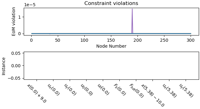
_ = prob.plot_constraint_violations(solution)
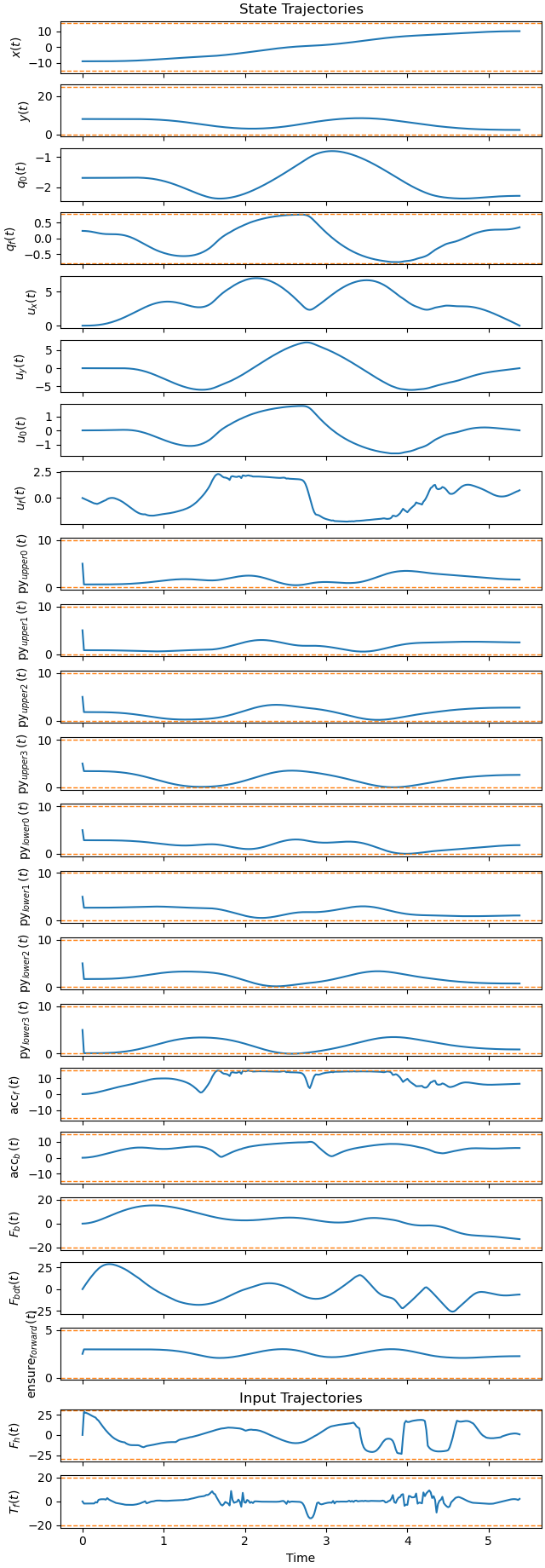
Plot generalized coordinates / speeds and forces / torques
_ = prob.plot_trajectories(solution, show_bounds=True)
Set Up the Limitation on the Energy in a Time Interval
For some reason, e.g. the battery driving the motor must not overheat, one wants to restrict this quantity
\(W_{\text{diff}} = \int_{t - \Delta}^{t} \max{(0, P(s))} ds \leq W_{max}\)
Here \(P(t) = \vec{F_b(t)} \circ \vec{v(t)}\), where \(\vec{F_b}\) drives the vehicle and \(\vec{v}\) is its speed. Neville Nieman (private communication) found a smooth approximation. \(S(x) \approx \max{(0, x)}\)
So
\(W_{\text{diff}} \approx \int_{t - \Delta}^{t} S(\vec{F_b} \circ \vec{v})(s) ds\)
\(= \int_0^t S(\vec{F_b}, \vec{v}) ds - \int_0^t S(\vec{F_b} \circ \vec{v})(s - \Delta) ds\)
\(= W(t) - W_{\text{delay}}\)
with
\(W_{\text{delay}} = \int_0^t S(\vec{F_b} \circ \vec{v})(s - \Delta) ds\)
\(= \int_0^{t - \Delta} S(\vec{F_b} \circ \vec{v})(s) ds\)
The idea was to make \(W_{\text{delay}}\) a numerical trajectory. For a numerical trajectory, one also needs its derivative w.r.t its variables, here: \(F_b, u_x, u_y, q_0\) The idea is:
\(\dfrac{d}{dt} W_{\text{delay}} = S(\vec{F_b} \circ\vec{v})(t)\)
hence
\(\dfrac{\partial}{\partial{F_b}} \dfrac{d}{dt}W_{\text{delay}} = \dfrac{\partial}{\partial{F_b}} S(\vec{F_b} \circ \vec{v})(t)\)
\(\dfrac{\partial}{\partial{F_b}} W_{\text{delay}} = \dfrac{\partial}{\partial{F_b}} \left[ \int_0^t S(\vec{F_b} \circ \vec{v})(s - \Delta) ds \right]\)
The last equation assumes that integration and differentiation may be exchanged. It should be the derivative needed, and similar for the other variables.
Note: \(F_b\) is the variable, \(\vec{F_b} = F_b \cdot Ab.y\)
time_delay = 1.0
sharpness = 1.0
W = me.dynamicsymbols('W')
W_diff = me.dynamicsymbols('W_diff')
W_delay_Fb = sm.symbols('W_delay', cls=sm.Function)(Fb)
WdtdFb = me.dynamicsymbols('WdtdFb')
WdFb = me.dynamicsymbols('WdFb')
W_delay_q0 = sm.symbols('W_delay_q0', cls=sm.Function)(q0)
Wdtdq0 = me.dynamicsymbols('Wdtdq0')
Wdq0 = me.dynamicsymbols('Wdq0')
W_delay_ux = sm.symbols('W_delay_ux', cls=sm.Function)(ux)
Wdtdux = me.dynamicsymbols('Wdtdux')
Wddux = me.dynamicsymbols('Wddux')
W_delay_uy = sm.symbols('W_delay_uy', cls=sm.Function)(uy)
Wdtduy = me.dynamicsymbols('Wdtduy')
Wdduy = me.dynamicsymbols('Wdduy')
power = Fb*Ab.y.dot(ux*N.x + uy*N.y)
ddt_W_func = 1 / sharpness * sm.ln(sm.exp(sharpness * power) + 1)
Add delay equations to the equations of motion.
verzoeg = sm.Matrix([
W.diff(t) - ddt_W_func,
W_diff - (W - W_delay_Fb),
WdtdFb - ddt_W_func.diff(Fb),
WdFb.diff(t) - WdtdFb,
Wdtdq0 - ddt_W_func.diff(q0),
Wdq0.diff(t) - Wdtdq0,
Wdtdux - ddt_W_func.diff(ux),
Wddux.diff(t) - Wdtdux,
Wdtduy - ddt_W_func.diff(uy),
Wdduy.diff(t) - Wdtduy,
])
eom = eom.col_join(verzoeg)
print(f'eom too large to print out. Its shape is '
f'{eom.shape} and it has ' +
f'{sm.count_ops(eom)} operations')
print(f"eom contains the following free symbols: {eom.free_symbols}")
print(f"eom depends on the following dynamic symbols: "
f"{me.find_dynamicsymbols(eom)}")
eom too large to print out. Its shape is (31, 1) and it has 877 operations
eom contains the following free symbols: {l, t, mb, mf, iZZb, iZZf, d, iZZ0, b, a, c, mh, reibung, m0}
eom depends on the following dynamic symbols: {u_f(t), Derivative(q_0(t), t), q_f(t), F_h(t), u_y(t), Derivative(WdFb(t), t), Wdduy(t), W_diff(t), Derivative(Wdq0(t), t), Derivative(F_b(t), t), ensure_forward(t), py_lower2(t), Derivative(q_f(t), t), Derivative(u_f(t), t), Derivative(Wdduy(t), t), W(t), u_0(t), x(t), Derivative(W(t), t), Derivative(Wddux(t), t), Derivative(u_0(t), t), T_f(t), Derivative(u_x(t), t), F_b(t), Derivative(y(t), t), Derivative(F_bdt(t), t), Derivative(u_y(t), t), Wdq0(t), acc_f(t), F_bdt(t), py_lower3(t), py_upper0(t), q_0(t), Wddux(t), Wdtduy(t), Wdtdux(t), y(t), py_upper1(t), u_x(t), WdFb(t), Derivative(x(t), t), py_upper2(t), py_lower1(t), W_delay(F_b(t)), py_lower0(t), acc_b(t), Wdtdq0(t), WdtdFb(t), py_upper3(t)}
Define the numerical trajectories for W_delay.
free_order = (
[x, y, q0, qf, ux, uy, u0, uf] +
py_upper + py_lower +
[acc_f, acc_b, Fb, Fbdt, ensure_forward] +
[W, W_diff,
WdFb, WdtdFb,
Wdq0, Wdtdq0,
Wddux, Wdtdux,
Wdduy, Wdtduy,
Fh, Tf, h,
]
)
def W_delay_traj(free):
time = np.linspace(0, free[-1] * (num_nodes - 1), num_nodes)
delayed_time = np.clip(time - time_delay, 0, None)
W_index = free_order.index(W)
W_arr = free[W_index * num_nodes: (W_index + 1) * num_nodes]
W_delay_arr = np.interp(delayed_time, time, W_arr)
return W_delay_arr
def WdFb_delay_traj(free):
time = np.linspace(0, free[-1] * (num_nodes - 1), num_nodes)
delayed_time = np.clip(time - time_delay, 0, None)
WdFb_index = free_order.index(WdFb)
WdFb_arr = free[WdFb_index * num_nodes: (WdFb_index + 1) * num_nodes]
WdFb_delay_arr = np.interp(delayed_time, time, WdFb_arr)
return WdFb_delay_arr
def Wdq0_delay_traj(free):
time = np.linspace(0, free[-1] * (num_nodes - 1), num_nodes)
delayed_time = np.clip(time - time_delay, 0, None)
Wdq0_index = free_order.index(Wdq0)
Wdq0_arr = free[Wdq0_index * num_nodes: (Wdq0_index + 1) * num_nodes]
Wdq0_delay_arr = np.interp(delayed_time, time, Wdq0_arr)
return Wdq0_delay_arr
def Wddux_delay_traj(free):
time = np.linspace(0, free[-1] * (num_nodes - 1), num_nodes)
delayed_time = np.clip(time - time_delay, 0, None)
Wddux_index = free_order.index(Wddux)
Wddux_arr = free[Wddux_index * num_nodes: (Wddux_index + 1) * num_nodes]
Wddux_delay_arr = np.interp(delayed_time, time, Wddux_arr)
return Wddux_delay_arr
def Wdduy_delay_traj(free):
time = np.linspace(0, free[-1] * (num_nodes - 1), num_nodes)
delayed_time = np.clip(time - time_delay, 0, None)
Wdduy_index = free_order.index(Wdduy)
Wdduy_arr = free[Wdduy_index * num_nodes: (Wdduy_index + 1) * num_nodes]
Wdduy_delay_arr = np.interp(delayed_time, time, Wdduy_arr)
return Wdduy_delay_arr
known_traj_map = {
W_delay_Fb: W_delay_traj,
W_delay_Fb.diff(Fb): WdFb_delay_traj,
W_delay_q0.diff(q0): Wdq0_delay_traj,
W_delay_ux.diff(ux): Wddux_delay_traj,
W_delay_uy.diff(uy): Wdduy_delay_traj,
}
Set Up the Second Optimization Problem and Solve it
t0 = 0.0
interval_value = h
tf = h * (num_nodes - 1)
state_symbols = (
[x, y, q0, qf, ux, uy, u0, uf] +
py_upper +
py_lower +
[acc_f, acc_b] + [Fb, Fbdt, ensure_forward] +
[W, W_diff,
WdFb, WdtdFb,
Wdq0, Wdtdq0,
Wddux, Wdtdux,
Wdduy, Wdtduy,
]
)
instance_constraints = (
W.func(t0),
W_diff.func(t0),
x.func(t0) + 9.0,
ux.func(t0),
uy.func(t0),
u0.func(t0),
uf.func(t0),
Fb.func(t0),
Fbdt.func(t0),
x.func(tf) - 10.0,
ux.func(tf),
uy.func(tf),
)
prob = Problem(
obj,
obj_grad,
eom,
state_symbols,
num_nodes,
interval_value,
known_parameter_map=par_map,
known_trajectory_map=known_traj_map,
instance_constraints=instance_constraints,
bounds=bounds,
backend='numpy',
time_symbol=t
)
Verify the free order matches extraction indices. This is needed for the known trajectories functions.
if list(prob._extraction_indices.keys()) != free_order:
print(f"used: {free_order}")
print(f"Correct: \n{list(prob._extraction_indices.keys())}")
raise ValueError("Free order does not match extraction indices.")
else:
print(f"Correct free_order:\n{free_order}")
Correct free_order:
[x(t), y(t), q_0(t), q_f(t), u_x(t), u_y(t), u_0(t), u_f(t), py_upper0(t), py_upper1(t), py_upper2(t), py_upper3(t), py_lower0(t), py_lower1(t), py_lower2(t), py_lower3(t), acc_f(t), acc_b(t), F_b(t), F_bdt(t), ensure_forward(t), W(t), W_diff(t), WdFb(t), WdtdFb(t), Wdq0(t), Wdtdq0(t), Wddux(t), Wdtdux(t), Wdduy(t), Wdtduy(t), F_h(t), T_f(t), h]
Solve the problem.
bounds = bounds | {W_diff: (-np.inf, 15.0)}
eom_bounds = {22: (-0.53, 0.53)}
prob = Problem(
obj,
obj_grad,
eom,
state_symbols,
num_nodes,
interval_value,
known_parameter_map=par_map,
known_trajectory_map=known_traj_map,
instance_constraints=instance_constraints,
bounds=bounds,
eom_bounds=eom_bounds,
backend='cython',
time_symbol=t
)
Create initial guess from the solution of the unrestricted problem.
s1 = solution
initial_guess = (list(s1[0: -2*num_nodes-1]) +
list(np.ones(10*num_nodes)) + list(s1[-2*num_nodes-1:-1]) +
[s1[-1]])
Solve the problem iteratively tightening the bounds on the difficult equation of motion.
fname1 = f'car_on_racecourse_limited_delay{num_nodes}_nodes_solution.csv'
start_zeit = time.time()
if os.path.exists(fname1):
# Take the existing solution.
solution = np.loadtxt(fname1)
else:
for i in range(4):
eom_bounds = {22: (-2.0 + i*0.49, 2.0 - i*0.49)}
prob = Problem(
obj,
obj_grad,
eom,
state_symbols,
num_nodes,
interval_value,
known_parameter_map=par_map,
known_trajectory_map=known_traj_map,
instance_constraints=instance_constraints,
bounds=bounds,
eom_bounds=eom_bounds,
backend='cython',
time_symbol=t,
tmp_dir='car_on_racecourse_opty_tempdir',
)
prob.add_option('max_iter', 30000)
solution, info = prob.solve(initial_guess)
initial_guess = solution
print(f'{i+1} - th iteration')
print('message from optimizer:', info['status_msg'])
print('Iterations needed', len(prob.obj_value))
print(f"objective value {info['obj_val']:.3e} \n")
#np.savetxt(fname1, solution, fmt='%.12f')
_ = prob.plot_objective_value()
end_zeit = time.time()
print(f'Time needed with delay: {end_zeit - start_zeit:.2f} sec')
Time needed with delay: 0.00 sec
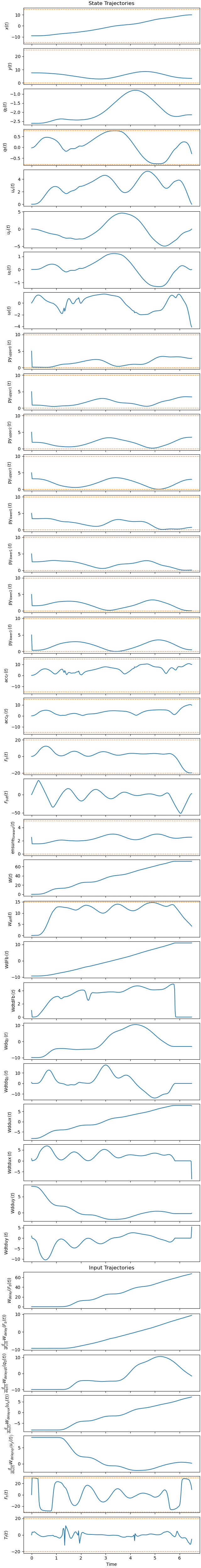
Print trajectories.
fig, ax = plt.subplots(38, 1, figsize=(6.4, 50), layout='constrained',
sharex=True)
_ = prob.plot_trajectories(solution, show_bounds=True, axes=ax)
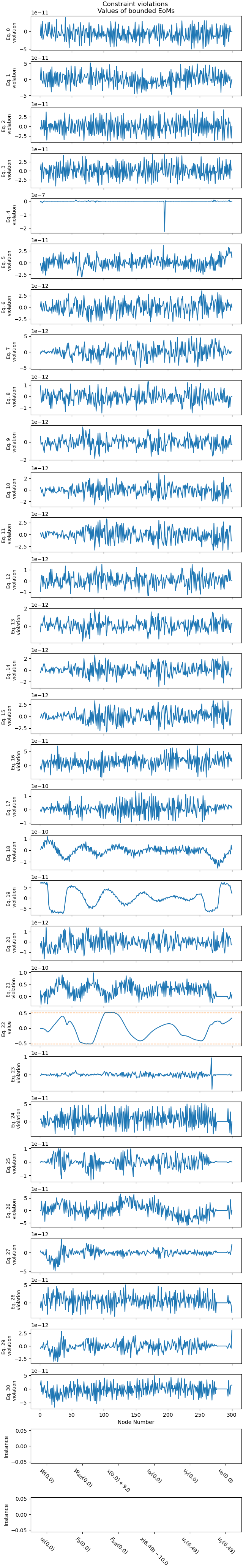
Plot constraint violations.
_ = prob.plot_constraint_violations(solution, subplots=True,
show_bounds=True)
Animate the Car
fps = 10
street_lam = sm.lambdify((x, a, b, c), street(x, a, b, c))
def add_point_to_data(line, x, y):
# to trace the path of the point. Copied from Timo.
old_x, old_y = line.get_data()
line.set_data(np.append(old_x, x), np.append(old_y, y))
state_vals, input_vals, _, h_vals = prob.parse_free(solution)
tf = solution[-1] * (num_nodes - 1)
t_arr = np.linspace(t0, tf, num_nodes)
state_sol = CubicSpline(t_arr, state_vals.T)
input_sol = CubicSpline(t_arr, input_vals.T)
# create additional points for the axles
Pbl, Pbr, Pfl, Pfr = sm.symbols('Pbl Pbr Pfl Pfr', cls=me.Point)
# end points of the force, length of the axles
Fbq = me.Point('Fbq')
la = sm.symbols('la')
fb, tq = sm.symbols('f_b, t_q')
Pbl.set_pos(Pb, -la/2 * Ab.x)
Pbr.set_pos(Pb, la/2 * Ab.x)
Pfl.set_pos(Pf, -la/2 * Af.x)
Pfr.set_pos(Pf, la/2 * Af.x)
Fbq.set_pos(Pb, Fb * Ab.y)
coordinates = Pb.pos_from(O).to_matrix(N)
for point in (Dmc, Pf, Pbl, Pbr, Pfl, Pfr, Fbq):
coordinates = coordinates.row_join(point.pos_from(O).to_matrix(N))
pL, pL_vals = zip(*par_map.items())
la1 = par_map[l] / 4. # length of an axle
la2 = la1/1.8
coords_lam = sm.lambdify((*state_symbols, tq, *pL, la), coordinates,
cse=True)
def init():
xmin, xmax = -13, 13.
ymin, ymax = -0.75, 12.5
fig = plt.figure(figsize=(8, 8))
ax = fig.add_subplot(111)
ax.set_xlim(xmin, xmax)
ax.set_ylim(ymin, ymax)
ax.set_aspect('equal')
ax.grid()
XX = np.linspace(xmin, xmax, 200)
ax.fill_between(XX, ymin,
street_lam(XX, par_map[a], par_map[b],
par_map[c] - la2), color='grey',
alpha=0.25)
ax.fill_between(XX,
street_lam(XX, par_map[a], par_map[b], par_map[c] +
par_map[d] + la2), ymax, color='grey',
alpha=0.25)
ax.plot(XX, street_lam(XX, par_map[a], par_map[b], par_map[c]-la2),
color='black')
ax.plot(XX, street_lam(XX, par_map[a],
par_map[b], par_map[c]+par_map[d]+la2), color='black')
ax.vlines(-10.0,
street_lam(-10.0, par_map[a], par_map[b], par_map[c]-la2),
street_lam(-10, par_map[a], par_map[b], par_map[c] +
par_map[d]+la2), color='red', linestyle='--')
ax.vlines(10.0, street_lam(10, par_map[a], par_map[b], par_map[c]-la2),
street_lam(10, par_map[a], par_map[b], par_map[c]+par_map[d] +
la2), color='green', linestyle='--')
line1, = ax.plot([], [], color='orange', lw=2)
line2, = ax.plot([], [], color='red', lw=2)
line3, = ax.plot([], [], color='magenta', lw=2)
line4 = ax.quiver([], [], [], [], color='green', scale=35,
width=0.004, headwidth=8)
return fig, ax, line1, line2, line3, line4
# Function to update the plot for each animation frame
fig, ax, line1, line2, line3, line4 = init()
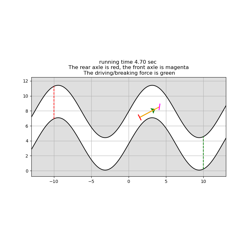
def update(t):
message = (f'running time {t:.2f} sec \n The rear axle is red, the ' +
f'front axle is magenta \n The driving/breaking force is green')
ax.set_title(message, fontsize=12)
coords = coords_lam(*state_sol(t), input_sol(t), *pL_vals, la1)
# Pb, Dmc, Pf, Pbl, Pbr, Pfl, Pfr, Fbq
line1.set_data([coords[0, 0], coords[0, 2]], [coords[1, 0], coords[1, 2]])
line2.set_data([coords[0, 3], coords[0, 4]], [coords[1, 3], coords[1, 4]])
line3.set_data([coords[0, 5], coords[0, 6]], [coords[1, 5], coords[1, 6]])
line4.set_offsets([coords[0, 0], coords[1, 0]])
line4.set_UVC(coords[0, 7] - coords[0, 0], coords[1, 7] - coords[1, 0])
frames = np.linspace(t0, tf, int(fps * (tf - t0)))
animation = FuncAnimation(fig, update, frames=frames, interval=1000/fps)
print(f'Total time needed: {time.time() - start_overall:.2f} sec')
Total time needed: 21.56 sec
fig, ax, line1, line2, line3, line4 = init()
update(4.7)
plt.show()
Total running time of the script: (0 minutes 30.377 seconds)