Particle on Numerical Surface

Objectives

• Show how to handle a numerical approximation of a function depending on more than one variable.

• Show how to handle derivatives of this numerical function when they appear in the equations of motion.

Description

A particle of mass \(m\) can slide on a surface described by a function \(\textrm{street}(x, y)\). The position of the particle is given by the coordinates \((x, y, \textrm{street}(x, y))\) in 3D space. The particle is subject to gravitation and speed dependent friction. A force \(\begin{pmatrix} f_x \\ f_y \\ f_z \end{pmatrix}\) acts on the particle, selected by opty. The goal is to go from A to B as fast as possible using minimal energy. The relative weight of speed vs. saving is determined by weight.

Explanations

1. Two sympy functions street_x(x) and street_y(y) are defined. They describe the same surface, but in street_x(x) x are considered variables and y are considered parameters - and vice versa.

2. Higher derivatives of street_x and street_y appear in the equations of motion. They are replaced by additional sympy functions like \(\dfrac{d}{dx} street_x(x) = \textrm{dstreet_x}(x)\) and \(\dfrac{d}{dy} street_y(y) = \textrm{dstreet_y}(y)\), etc.

3. For every numerical function given, opty needs it derivate w.r.t the variable. In this example \(\dfrac{d^3}{dx^3} street_x(x)\) and \(\dfrac{d^3}{dy^3} street_y(y)\) are needed. In a real world situation they would be the results of measurements.

States

• \(x, y\) : coordinates of the particle

• \(u_x, u_y\) : velocities of the particle

Parameters - \(m\) : mass of the particle - \(g\) : gravitational acceleration - \(\mu\) : speed dependentfriction coefficient - \(\omega_1, \omega_2\) : angular frequencies - \(a\) : amplitude

Controls - \(f_x, f_y, f_z\) : forces acting on the particle

Others

• \(\textrm{street_x}(x), \textrm{street_y}(y)\) : numerical functions

• \(\textrm{dstreet}_x\) : \(\dfrac{d}{dx} \textrm{street_x}(x)\)

• \(\textrm{dstreet}_y\) : \(\dfrac{d}{dy} \textrm{street_y}(y)\)

• \(\textrm{ddstreet}_x\) : \(\dfrac{d^2}{dx^2} \textrm{street_x}(x)\)

• \(\textrm{ddstreet}_y\) : \(\dfrac{d^2}{dy^2} \textrm{street_y}(y)\)

• \(\textrm{dddstreet}_x\) : \(\dfrac{d^3}{dx^3} \textrm{street_x}(x)\)

• \(\textrm{dddstreet}_y\) : \(\dfrac{d^3}{dy^3} \textrm{street_y}(y)\)

import numpy as np
import sympy as sm
import sympy.physics.mechanics as me
import matplotlib.pyplot as plt
from opty import Problem
from scipy.interpolate import CubicSpline
from matplotlib.animation import FuncAnimation

Kane’s Method

N = me.ReferenceFrame('N')
O, P = sm.symbols('O P', cls=me.Point)
t = me.dynamicsymbols._t
O.set_vel(N, 0)
P.set_vel(N, 0)

x, y, ux, uy = me.dynamicsymbols('x y u_x u_y')
street_x = sm.Function('street_x')(x)
street_y = sm.Function('street_y')(y)

dstreet_x = sm.Function('dstreet_x')(x)
dstreet_y = sm.Function('dstreet_y')(y)

ddstreet_x = sm.Function('ddstreet_x')(x)
ddstreet_y = sm.Function('ddstreet_y')(y)

Needed to replace derivatives in equations of motion with ‘new’ functions

street_dict = {
    street_x.diff(x): dstreet_x,
    street_y.diff(y): dstreet_y,
    street_x.diff(x, 2): ddstreet_x,
    street_y.diff(y, 2): ddstreet_y
}

fx, fy, fz = me.dynamicsymbols('f_x f_y f_z')
m, g, mu = sm.symbols('m g mu', real=True)

# As street_x, street_y describe the same surface, it does not matter which
# one is used here
P.set_pos(O, x * N.x + y * N.y + street_x * N.z)

# The speed in z direction is d/dt(surface(x, y)) = d/dt(street_x(x)) * ux +
# d/dt(street_y(y)) * uy
P.set_vel(N, ux * N.x + uy * N.y + (street_x.diff(x) * ux +
                                    street_y.diff(y) * uy) * N.z)

body = me.Particle('body', P, m)
bodies = [body]

force = [(P, fx * N.x + fy * N.y + fz * N.z - m * g * N.z - mu * P.vel(N))]

kd = sm.Matrix([ux - x.diff(t), uy - y.diff(t)])

q_ind = [x, y]
u_ind = [ux, uy]

KM = me.KanesMethod(N, q_ind, u_ind, kd)
fr, frstar = KM.kanes_equations(bodies, force)
eoms = me.msubs(kd.col_join(fr + frstar), street_dict)
print('eom dynamic symbols: ', me.find_dynamicsymbols(eoms), '\n')
print(F'eoms have {sm.count_ops(eoms)} operations')

eom dynamic symbols:  {u_x(t), ddstreet_y(y(t)), f_y(t), Derivative(u_y(t), t), f_z(t), y(t), dstreet_x(x(t)), Derivative(u_x(t), t), f_x(t), ddstreet_x(x(t)), Derivative(y(t), t), Derivative(x(t), t), u_y(t), dstreet_y(y(t)), x(t)}

eoms have 122 operations

Set Up the Optimisation and Solve It

h = sm.symbols('h', real=True)
num_nodes = 201
t0, tf = 0.0, (num_nodes - 1) * h
interval_value = h

state_symbols = [x, y, ux, uy]

Define the various functions needed in the known_trajectory_map. In a real situation they would be the results of measurements.

a, omega1, omega2 = sm.symbols('a omega_1 omega_2', real=True)


def strasse(x, y, a, omega1, omega2):
    return a * (sm.sin(omega1 * x) * sm.sin(omega2 * y))


par_map = {
    m: 1.0,
    g: 9.81,
    mu: 0.1,
    omega1: 2.0 * np.pi / 17.0,
    omega2: 2.0 * np.pi / 25.0,
    a: 4.0
}

street_xx = strasse(x, y, a, omega1, omega2)
street_yy = strasse(x, y, a, omega1, omega2)
dstreet_xx = street_xx.diff(x)
dstreet_yy = street_yy.diff(y)
ddstreet_xx = dstreet_xx.diff(x)
ddstreet_yy = dstreet_yy.diff(y)
dddstreet_xx = ddstreet_xx.diff(x)
dddstreet_yy = ddstreet_yy.diff(y)

x_meas = np.linspace(-10, 10, 1000)
y_meas = np.linspace(-10, 10, 1000)

street_x_lam = sm.lambdify((x, y), street_xx.subs(par_map), cse=True)
street_y_lam = sm.lambdify((x, y), street_yy.subs(par_map), cse=True)
dstreet_x_lam = sm.lambdify((x, y), dstreet_xx.subs(par_map), cse=True)
ddstreet_x_lam = sm.lambdify((x, y), ddstreet_xx.subs(par_map), cse=True)
dstreet_y_lam = sm.lambdify((x, y), dstreet_yy.subs(par_map), cse=True)
ddstreet_y_lam = sm.lambdify((x, y), ddstreet_yy.subs(par_map), cse=True)
dddstreet_x_lam = sm.lambdify((x, y), dddstreet_xx.subs(par_map), cse=True)
dddstreet_y_lam = sm.lambdify((x, y), dddstreet_yy.subs(par_map), cse=True)

street_x_meas = street_x_lam(x_meas, y_meas)
street_y_meas = street_y_lam(x_meas, y_meas)
dstreet_x_meas = dstreet_x_lam(x_meas, y_meas)
ddstreet_x_meas = ddstreet_x_lam(x_meas, y_meas)
dstreet_y_meas = dstreet_y_lam(x_meas, y_meas)
ddstreet_y_meas = ddstreet_y_lam(x_meas, y_meas)
dddstreet_x_meas = dddstreet_x_lam(x_meas, y_meas)
dddstreet_y_meas = dddstreet_y_lam(x_meas, y_meas)


def calc_street_x(free):
    x = free[0: num_nodes]
    return np.interp(x, x_meas, street_x_lam(x_meas, y_meas))


def calc_street_y(free):
    y = free[num_nodes: 2 * num_nodes]
    return np.interp(y, x_meas, street_y_lam(x_meas, y_meas))


def calc_dstreet_x(free):
    x = free[0: num_nodes]
    return np.interp(x, x_meas, dstreet_x_lam(x_meas, y_meas))


def calc_dstreet_y(free):
    y = free[num_nodes: 2 * num_nodes]
    return np.interp(y, x_meas, dstreet_y_lam(x_meas, y_meas))


def calc_ddstreet_x(free):
    x = free[0: num_nodes]
    return np.interp(x, x_meas, ddstreet_x_lam(x_meas, y_meas))


def calc_ddstreet_y(free):
    y = free[num_nodes: 2 * num_nodes]
    return np.interp(y, x_meas, ddstreet_y_lam(x_meas, y_meas))


def calc_dddstreet_x(free):
    x = free[0: num_nodes]
    return np.interp(x, x_meas, dddstreet_x_lam(x_meas, y_meas))


def calc_dddstreet_y(free):
    y = free[num_nodes: 2 * num_nodes]
    return np.interp(y, x_meas, dddstreet_y_lam(x_meas, y_meas))

Finish setting up the optimization problem.

instance_constraints = [
    x.func(t0) + 9.0,
    y.func(t0) + 9.0,
    ux.func(t0),
    uy.func(t0),
    # values on fx, fy, fz to avoid division by zero warning when plotting.
    fx.func(t0) - 1.e-10,
    fy.func(t0) - 1.e-10,
    fz.func(t0) - 1.e-10,
    x.func(tf) - 9.0,
    y.func(tf) - 9.0,
    ux.func(tf),
    uy.func(tf),
]

limit = 20.0
bounds = {
    fx: (-limit, limit),
    fy: (-limit, limit),
    fz: (-limit, limit),
    h: (0.0, 0.5),
}

weight = 900


def obj(free):
    summe = (np.sum(free[4 * num_nodes: 7 * num_nodes]**2) * free[-1] +
             weight * free[-1])
    return summe


def obj_grad(free):
    grad = np.zeros_like(free)
    grad[4 * num_nodes: 7 * num_nodes] = 2.0 * free[4 * num_nodes: 7 *
                                                    num_nodes] * free[-1]
    grad[-1] = np.sum(free[4 * num_nodes: 7 * num_nodes]**2) + weight
    return grad


prob = Problem(
    obj,
    obj_grad,
    eoms,
    state_symbols,
    num_nodes,
    interval_value,
    known_parameter_map=par_map,
    known_trajectory_map={
        street_x: calc_street_x,
        street_x.diff(x): calc_dstreet_x,
        street_y: calc_street_y,
        street_y.diff(y): calc_dstreet_y,
        dstreet_x: calc_dstreet_x,
        dstreet_x.diff(x): calc_ddstreet_x,
        dstreet_y: calc_dstreet_y,
        dstreet_y.diff(y): calc_ddstreet_y,
        ddstreet_x: calc_ddstreet_x,
        ddstreet_x.diff(x): calc_dddstreet_x,
        ddstreet_y: calc_ddstreet_y,
        ddstreet_y.diff(y): calc_dddstreet_y,
        },
    instance_constraints=instance_constraints,
    bounds=bounds,
    time_symbol=t,
#    backend='numpy',
)

Solve the optimization problem.

initial_guess = np.zeros(prob.num_free)
x_guess = np.linspace(-8.0, 8.0, num_nodes)
y_guess = np.linspace(-8.0, 8.0, num_nodes)
initial_guess[0:num_nodes] = x_guess  # x
initial_guess[num_nodes:2 * num_nodes] = y_guess  # y
initial_guess[-1] = 0.01  # h

prob.add_option('max_iter', 6000)
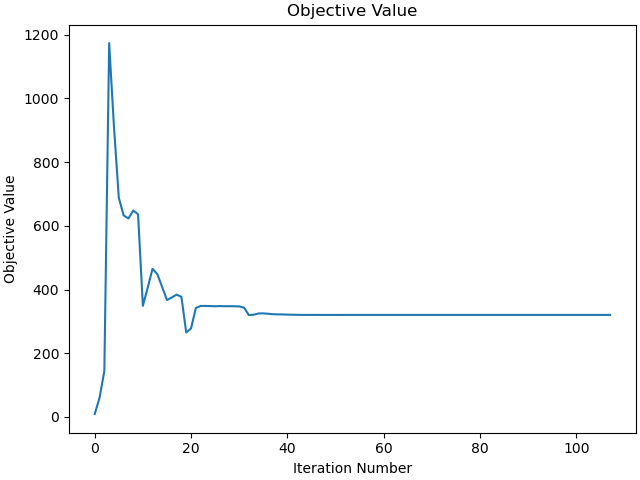
solution, info = prob.solve(initial_guess)
initial_guess = solution
print(info['status_msg'])
print(info['obj_val'])

b'Algorithm stopped at a point that was converged, not to "desired" tolerances, but to "acceptable" tolerances (see the acceptable-... options).'
320.1878509073637

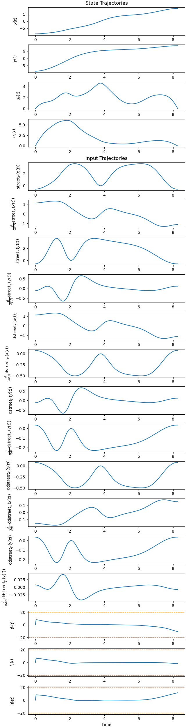
Plot trajectories.

fig, ax = plt.subplots(19, 1, figsize=(6.4, 25), layout='constrained')
_ = prob.plot_trajectories(solution, axes=ax, show_bounds=True)

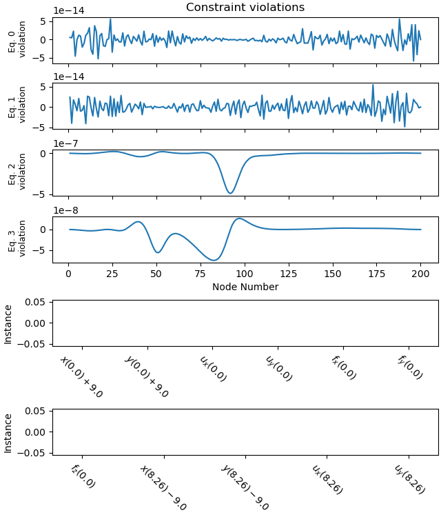
Plot errors.

_ = prob.plot_constraint_violations(solution, subplots=True)

Plot objective value.

_ = prob.plot_objective_value()

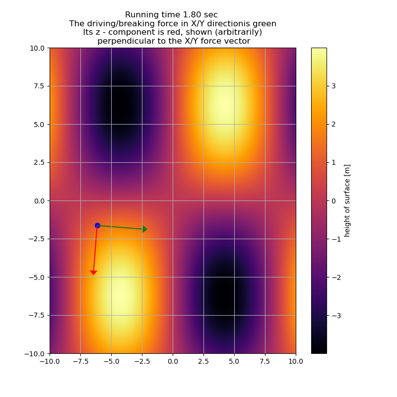
Animation

fps = 2.5
street_lam = street_x_lam

state_vals, input_vals, _, h_vals = prob.parse_free(solution)
tf = h_vals * (num_nodes - 1)
t_arr = np.linspace(t0, tf, num_nodes)
state_sol = CubicSpline(t_arr, state_vals.T)
input_sol = CubicSpline(t_arr, input_vals.T)

# end points of the force
Fbq, Fbz = me.Point('Fbq'), me.Point('Fbz')
sx, sy = sm.symbols('sx, sy', real=True)

Fbq.set_pos(P, fx * N.x + fy * N.y)
# A unit vector normal to fx * N.x + fy * N.y is
# v = (fy, -fx) * 1 / sqrt(fx**2 + fy**2)
Fbz.set_pos(P, fz / sm.sqrt(fx**2 + fy**2) * (fy * N.x - fx * N.y))

coordinates = P.pos_from(O).to_matrix(N)
coordinates = coordinates.row_join(Fbq.pos_from(O).to_matrix(N))
coordinates = coordinates.row_join(Fbz.pos_from(O).to_matrix(N))
coordinates = coordinates.subs({street_x: sx, street_y: sy})

pL, pL_vals = zip(*par_map.items())
coords_lam = sm.lambdify((*state_symbols, fx, fy, fz, sx, sy, *pL),
                         coordinates, cse=True)


def init():
    xmin, xmax = -10., 10.
    ymin, ymax = -10, 10

    fig = plt.figure(figsize=(8, 8))
    ax = fig.add_subplot(111)
    ax.set_xlim(xmin, xmax)
    ax.set_ylim(ymin, ymax)
    ax.set_aspect('equal')
    ax.grid()

    # Create grid of x, y points
    X, Y = np.meshgrid(x_meas, y_meas)

    Z = street_x_lam(X, Y)  # Calculate z values using the street function

    # Plot the colored surface
    ax.pcolormesh(X, Y, Z, shading='auto', cmap='inferno')
    c = ax.imshow(Z, extent=[x_meas.min(), x_meas.max(), y_meas.min(),
                             y_meas.max()], origin='lower', cmap='inferno',
                  aspect='auto')

    fig.colorbar(c, ax=ax, label="height of surface [m]")

    line1 = ax.scatter(-8.0, -8.0, color='blue', s=50)
    pfeil = ax.quiver([], [], [], [], color='green', scale=10,
                      width=0.004, headwidth=8)
    pfeil_z = ax.quiver([], [], [], [], color='red', scale=10,
                        width=0.004, headwidth=8)

    return fig, ax, line1, pfeil, pfeil_z


# Function to update the plot for each animation frame
fig, ax, line1, pfeil, pfeil_z = init()


def update(t):
    message = ((f'Running time {t:.2f} sec \n '
                f'The driving/breaking force in X/Y directionis green \n '
                f'Its z - component is red, shown (arbitrarily) \n '
                f'perpendicular to the X/Y force vector'))
    ax.set_title(message, fontsize=12)

    sx = street_x_lam(*state_sol(t)[0: 2])
    sy = sx
    coords = coords_lam(*state_sol(t), *input_sol(t), sx, sy, *pL_vals)

    line1.set_offsets([coords[0, 0], coords[1, 0]])
    pfeil.set_offsets([coords[0, 0], coords[1, 0]])
    pfeil.set_UVC(coords[0, 1] - coords[0, 0], coords[1, 1] - coords[1, 0])
    pfeil_z.set_offsets([coords[0, 0], coords[1, 0]])
    pfeil_z.set_UVC(coords[0, 2] - coords[0, 0], coords[1, 2] - coords[1, 0])


frames = np.linspace(t0, tf, int(fps * (tf - t0)))
animation = FuncAnimation(fig, update, frames=frames, interval=1000/fps)

Once Loop Reflect

fig, ax, line1, pfeil, pfeil_z = init()
update(1.8)

plt.show()