Note
Go to the end to download the full example code.
Colliding Discs
Objectives
Show how to model impacts using Hunt-Crossley’s theory
Show how to handle a somewhat non-trivial system using Kane’s method in sympy.physics.mechanics
Description
n discs, named \(Dmc_0....Dmc_{n-1}\) with radius \(r_0\) and mass \(m_0\) are sliding frictionlessly on the horizontal X/Z plane.
Their space is limited by a circular wall of radius \(R_W\) and center at the origin of the inertial frame \(N\), which is fixed in space.
The collision force is always on the line \(\overline{Dmc_i, Dmc_j}\), \(0 \le i, j \le n-1\), \(i \neq j\), or on a line perpendicular to the tangent of the circular wall at the collision point. Of course, this line will go through Dmc[i] There is speed dependent friction between discs, with coefficient \(m_u\) and between wall and discs, with coefficient \(m_{uW}\)
An observer, a particle of mass \(m_o\) may be attached anywhere within each disc.
Note about the force during the collisions
Hunt Crossley’s method
Reference is this article: https://www.sciencedirect.com/science/article/pii/S0094114X23000782
This is with dissipation during the collision, the general force is given in (63) of the article as:\(f_n = k_0 \cdot \rho + \chi \cdot \dot \rho\), with \(k_0\) as below, \(\rho\) the penetration, and \(\dot\rho\) the speed of the penetration. In the article it is stated, that \(n = \frac{3}{2}\) is a good choice, it is derived in Hertz’ approach. Of course, \(\rho, \dot\rho\) must be the signed magnitudes of the respective vectors. A more realistic force is given in (64) as: \(f_n = k_0 \cdot \rho^n + \chi \cdot \rho^n\cdot \dot \rho\), as this avoids discontinuity at the moment of impact. Hunt and Crossley give this value for \(\chi\), see table 1:
\(\chi = \dfrac{3}{2} \cdot(1 - c_\tau) \cdot \dfrac{k_0}{\dot \rho^{(-)}}\), where \(c_\tau = \dfrac{v_1^{(+)} - v_2^{(+)}}{v_1^{(-)} - v_2^{(-)}}\), where \(v_i^{(-)}, v_i^{(+)}\) are the speeds of \(body_i\), before and after the collosion, see (45), \(\dot\rho^{(-)}\) is the speed right at the time the impact starts. \(c_\tau\) is an experimental factor, apparently around 0.8 for steel.
Using (64), this results in their expression for the force:
\(f_n = k_0 \cdot \rho^n \left[1 + \dfrac{3}{2} \cdot(1 - c_\tau) \cdot \dfrac{\dot\rho}{\dot\rho^{(-)}}\right]\)
with \(k_0 = \frac{4}{3\cdot(\sigma_1 + \sigma_2)} \cdot \sqrt{\frac{R_1 \cdot R_2}{R_1 + R_2}}\),
where
\(\sigma_i = \frac{1 - \nu_i^2}{E_i}\),
with
\(\nu_i\) = Poisson’s ratio, \(E_i\) = Young”s modulus, \(R_1, R_2\) the radii of the colliding bodies, \(\rho\) the penetration depth.
All is near equations (54) and (61) of this article.
As per the article, \(n = \frac{3}{2}\) is always to be used.
spring energy = \(k_0 \cdot \int_{0}^{\rho} k^{3/2}\,dk = k_0 \cdot\frac{2}{5} \cdot \rho^{5/2}\) I assume, the dissipated energy cannot be given in closed form, at least the article does not give one.
Notes
\(c_\tau = 1.\) gives Hertz’s solution to the impact problem, also described in the article.
From the discs’ point of view, the wall is concave. I model this by taking \(R_2 = -R_W\). As \(|R_1| < |R_2|\) this should give no issues. I do not know, whether this approach is theoretically correct.
Variables
\(n\): number of discs
\(m_0\): mass of the discs
\(m_o\): mass of the observer
\(r_0\): radius of the discs
\(R_W\): radius of the wall
\(k_0\): modulus of elasticity of the pendulum body
\(k_{0W}\): modulus of elasticity of the collision disc with a wall
\(i_{YY_i}\): moment of inertia of the i-th disc
\(c_\tau\): the experimental constant needed for Hunt-Crossley
\(m_u\): coefficient of friction between discs / between disc and wall
\(m_{uW}\): coefficient of friction between disc and wall
\(t\): time
\(q_0...q_{n-1}\): generalized coordinates for the discs
\(u_0...u_{n-1}\): the angular speeds
\(x_i, z_i\): the coordinates, in the inertial frame \(N\), of the center of the i-th disc
\(ux_i, uz_i\): their speeds
\(N\): frame of inertia
\(P_0\): point fixed in \(N\)
\(A_i\): body fixed frame of the i-th disc
\(Dmc_i\): center of the i-th disc
\(Po_i\): observer (particle) on i-th disc
\(\alpha_i\): distance of observer on i-th disc
\(CP_i\): contact point of \(disc_i\) with the wall
\(rhodt_{max}\): the collission speed, to be determined during integration, needed for Hunt-Crossley
import sympy.physics.mechanics as me
import sympy as sm
from scipy.integrate import solve_ivp
import numpy as np
from itertools import permutations
import matplotlib.pyplot as plt
from matplotlib import animation
import matplotlib as mp
This is needed to exit a loop, when a feasible initial location of the discs within the limitations of the wall was found.
class Rausspringen(Exception):
pass
Kane’s Equations of Motion
Set up some of the geometry.
n = 3 # Number of discs, must be larger than 1
if isinstance(n, int) is False or n < 2:
raise Exception('n must be an integer larger than 1')
q_list = me.dynamicsymbols(f'q:{n}')
u_list = me.dynamicsymbols(f'u:{n}')
x_list = me.dynamicsymbols(f'x:{n}')
z_list = me.dynamicsymbols(f'z:{n}')
ux_list = me.dynamicsymbols(f'ux:{n}')
uz_list = me.dynamicsymbols(f'uz:{n}')
CPx_list = list(sm.symbols(f'CPx:{n}'))
CPz_list = list(sm.symbols(f'CPz:{n}'))
CP_list = list(sm.symbols(f'CP:{n}', cls=me.Point))
rhodtmax = []
for i, j in permutations(range(n), r=2):
rhodtmax.append(sm.symbols('rhodtmax' + str(i) + str(j)))
rhodtwall = list(sm.symbols(f'rhodtwall:{n}'))
m0, mo, r0, RW, k0, k0W, iYY, ctau, mu, muW = sm.symbols('m0, mo, r0, RW, k0,'
'k0W, iYY, ctau, mu,'
'muW')
N = me.ReferenceFrame('N')
P0 = me.Point('P0')
P0.set_vel(N, 0)
t = me.dynamicsymbols._t
A_list = sm.symbols(f'A:{n}', cls=me.ReferenceFrame)
Dmc_list = sm.symbols(f'Dmc:{n}', cls=me.Point)
Po_list = sm.symbols(f'Po:{n}', cls=me.Point)
CP_list = list(sm.symbols(f'CP:{n}', cls=me.Point))
alpha_list = sm.symbols(f'alpha:{n}')
Body1 = []
Body2 = []
for i in range(n):
A_list[i].orient_axis(N, q_list[i], N.y)
A_list[i].set_ang_vel(N, u_list[i] * N.y)
Dmc_list[i].set_pos(P0, x_list[i]*N.x + z_list[i]*N.z)
Dmc_list[i].set_vel(N, ux_list[i]*N.x + uz_list[i]*N.z)
Po_list[i].set_pos(Dmc_list[i], r0 * alpha_list[i] * A_list[i].x)
Po_list[i].v2pt_theory(Dmc_list[i], N, A_list[i])
CP_list[i].set_pos(P0, CPx_list[i]*N.x + CPz_list[i]*N.z)
I = me.inertia(A_list[i], 0, iYY, 0)
body = me.RigidBody('body' + str(i), Dmc_list[i], A_list[i], m0,
(I, Dmc_list[i]))
teil = me.Particle('teil' + str(i), Po_list[i], mo)
Body1.append(body)
Body2.append(teil)
BODY = Body1 + Body2
Colliding force between discs
This function returns the force, as given by Hunt-Crossley, which \(P_1\) excerts on \(P_2\). The relevant speed is only the speed component in \(\overline{P_1 P_2}\) direction. \(sm.Heaviside(2. \cdot r - abstand, 0)\) ensures, that there is a force only during the collision.
I get \(\dot\rho^{(-)}\) during integration. The way I defined it, it should always be negative, just like \(\dot\rho\) in the first phase of the penetration. For whatever reason, this is not always so. Using \(\dfrac{-\dot\rho}{|\dot\rho^{(-)}|}\) gives the right results.
def HC_disc(N, P1, P2, r, ctau, rhodtmax, k0):
'''
Calculates the contact force exerted by P1 on P2, according to the
Hunt-Crossley formula given above.
I assume, that the contact force always acts along the line P1/P2.
I think, this is a fair assymption if the colliding balls are homogenious.
The variables in the list are
- N is an me.ReferenceFrame, the inertial frame
- P1, P2 are me.Point objects. They are the centers of two me.RigidBody
objects, here assumed to be two ball each of radius r
- radius of the ball
- ctau, the experimental constant needed
- rhodtmax, the relative speeds of P1 to P2, right at the impact time,
measured in N.
This has to be calculated numerically during the integration.
- k0 is the force constant
'''
vektorP1P2 = P2.pos_from(P1)
abstand = vektorP1P2.magnitude()
richtung = vektorP1P2.normalize()
# penetration. Positive if the two balls are in collision
rho = (2.*r - abstand)/2.
geschw = vektorP1P2.diff(t, N)
rhodt = me.dot(geschw, richtung)
rho = sm.Max(rho, sm.S(0)) # if rho < 0., rho**(3/2) will give problems
kraft = (k0 * rho**(3/2) * (1. + 3./2. * (1 - ctau) *
(-rhodt/sm.Abs(rhodtmax))) *
sm.Heaviside(2. * r - abstand, 0.) * richtung)
return kraft
Collision force between disc and the wall As far as the penetration depth is concerned, this is like two discs colliding: the penetration depth of the wall into the disc is the same as the disc into the wall.
def HC_wall(N, P1, CP, r, ctau, rhodtwall, k0W):
'''
Calculates the contact force exerted by the wall on P1, according to the
Hunt-Crossley formula given above. I assume, that the contact force always
acts in the direction normal to the tangent of the wall at the
collision point CP.
The variables in the list are
- N is an me.ReferenceFrame, the inertial frame
- P1, is a me.Point object, the center of the disc
- CP is the point where the disc collides with the wall.
- radius of the disc
- ctau, the experimental constant needed
- rhodtmax, a list containing the speed right before P1 hits wall_i
This has to be calculated numerically during the integration.
- k0W is the force constant. This is different from k0 as the wall is like a
disc with R = -RW.
'''
vektor = P1.pos_from(CP)
abstand = vektor.magnitude()
richtung = vektor.normalize()
# penetration. Positive if the disc is in collision with the wall
rho = (r - abstand)
rhodt = me.dot(P1.vel(N), richtung)
rho = sm.Max(rho, sm.S(0)) # if rho < 0., rho**(3/2) will give problems
kraft0 = (k0W * rho**(3/2) * (1. + 3./2. * (1 - ctau)
* (-rhodt/sm.Abs(rhodtwall)))
* sm.Heaviside(r - abstand, 0.) * richtung)
return kraft0
Friction when a disc hits another disc
This website: https://math.stackexchange.com/questions/2195047/solve-the-vector-cross-product-equation
gives: \(b = a \times x \rightarrow x = \dfrac{b \times a}{|a|^2}\)
This way, one can easily get the force acting on P1, without any further geometric considerations.
def friction_disc(N, A1, A2, P1, P2, r, ctau, rhodtmax, k0, mu):
'''
when two discs collide, their surface speed in general will be different.
There is a force caused by friction. Here I calculate the force acting on the
contact point CP1 of P1 in direction of the tangent on disc1, whose center is
P1, proportional to v(CP2) - v(CP1)
* the magnitude of the collision force which P2 excerts on P1
* the coefficient of friction mu
The force on CP is equivalent to a force on Dmc and a torque on A
'''
CPa, CPb = sm.symbols('CPa, CPb', cls=me.Point)
abstand = P2.pos_from(P1)
CPa.set_pos(P1, abstand / 2.)
CPa.v2pt_theory(P1, N, A1)
CPb.set_pos(P2, -abstand / 2.)
CPb.v2pt_theory(P2, N, A2)
delta_v = CPb.vel(N) - CPa.vel(N)
force_coll = HC_disc(N, P2, P1, r, ctau, rhodtmax, k0).magnitude()
force_fric = (force_coll * mu * delta_v)
torque = (0.5 * abstand.cross(force_fric) *
sm.Heaviside(2. * r - abstand.magnitude()))
kraft = (1./(0.25 * me.dot(abstand, abstand)) * torque.cross(abstand) *
sm.Heaviside(2. * r - abstand.magnitude()))
return [kraft, torque]
Friction when a disc hits the wall
def friction_wall(N, A1, P1, CP, r, ctau, rhodtwall, k0W, mu):
'''
When a disc collides with a wall, there will be a force due to friction.
I calculate the force due to friction on the contact point CP1.
This force is parallel to the wall, and proportional to
* the speed of CP1
* the magnitude of the collision force
* the coefficient of friction mu
'''
vektor = P1.pos_from(CP)
abstand = vektor.normalize()
CPa = me.Point('CPa')
CPa.set_pos(P1, -abstand)
CPa.v2pt_theory(P1, N, A1)
force_coll = HC_wall(N, P1, CP, r, ctau, rhodtwall, k0W).magnitude()
force_fric = -force_coll * mu * CPa.vel(N)
torque0 = (CPa.pos_from(P1).cross(force_fric) *
sm.Heaviside(r - vektor.magnitude()))
kraft0 = (1./me.dot(abstand, abstand) * torque0.cross(-abstand) *
sm.Heaviside(r - vektor.magnitude()))
return [kraft0, torque0]
force from the collision of discs with discs and discs with the wall
With permutations(range(n), r=2) I get all possible forces of \(disc_j\) on \(disc_i\), \(0 \le i, j \le n-1, i \neq j\) This is not the most efficient way to do it, as for example \(F^{disc_i \space \backslash \space disc_j} = -F^{disc_j \space \backslash \space disc_i}\), but this way seems easier to keep it all ‘straight’.
FL = []
# Hunt - Crossley type collision forces between discs and between disc and wall
zaehler = -1
for i, j in permutations(range(n), r=2):
zaehler += 1
FL.append((Dmc_list[i], HC_disc(N, Dmc_list[j], Dmc_list[i], r0,
ctau, rhodtmax[zaehler], k0)))
for i in range(n):
FL.append((Dmc_list[i], HC_wall(N, Dmc_list[i], CP_list[i], r0, ctau,
rhodtwall[i], k0W)))
# Friction forces between discs
zaehler = -1
for i, j in permutations(range(n), r=2):
zaehler += 1
FL.append((Dmc_list[i], friction_disc(N, A_list[i], A_list[j], Dmc_list[i],
Dmc_list[j], r0, ctau,
rhodtmax[zaehler], k0, mu)[0]))
FL.append((A_list[i], friction_disc(N, A_list[i], A_list[j], Dmc_list[i],
Dmc_list[j], r0, ctau,
rhodtmax[zaehler], k0, mu)[1]))
# Friction forces between disc and wall
for i in range(n):
FL.append((Dmc_list[i], friction_wall(N, A_list[i], Dmc_list[i],
CP_list[i], r0, ctau, rhodtwall[i],
k0W, muW)[0]))
FL.append((A_list[i], friction_wall(N, A_list[i], Dmc_list[i],
CP_list[i], r0, ctau, rhodtwall[i],
k0W, muW)[1]))
Kane’s equations
kd = [i - sm.Derivative(j, t) for i, j in zip(u_list + ux_list + uz_list,
q_list + x_list + z_list)]
q_ind = x_list + z_list + q_list
u_ind = ux_list + uz_list + u_list
KM = me.KanesMethod(N, q_ind=q_ind, u_ind=u_ind, kd_eqs=kd)
(fr, frstar) = KM.kanes_equations(BODY, FL)
MM = KM.mass_matrix_full
print('MM DS', me.find_dynamicsymbols(MM))
print('MM free symbols', MM.free_symbols)
print(f'MM contains {sm.count_ops(MM):,} operations')
force = KM.forcing_full
print('force DS', me.find_dynamicsymbols(force), '\n')
print('force free symbols', force.free_symbols, '\n')
print(f'force contains {sm.count_ops(force):,} operations', '\n')
MM DS {q1(t), q0(t), q2(t)}
MM free symbols {alpha1, r0, m0, alpha0, iYY, t, alpha2, mo}
MM contains 93 operations
force DS {z1(t), u2(t), q0(t), uz2(t), uz0(t), x2(t), uz1(t), ux0(t), x0(t), u0(t), z0(t), u1(t), q1(t), z2(t), x1(t), ux1(t), ux2(t), q2(t)}
force free symbols {r0, CPz2, CPz0, alpha0, rhodtmax21, rhodtmax12, rhodtmax20, k0W, CPx2, rhodtmax02, t, alpha2, mo, muW, rhodtmax01, alpha1, k0, rhodtwall1, mu, CPx1, rhodtmax10, rhodtwall2, ctau, rhodtwall0, CPx0, CPz1}
force contains 13,983 operations
Here various functions are defined, which are needed later.
rhomax_list: It is used during integration to calculate the speeds just before impact between \(disc_j\) and \(disc_i\), \(0 \le i, j \le n-1, i \neq j\)
rhowall_list: It is used during integration to calculate the speeds just before impact between \(disc_i\) and the walls.
Dmc_pos: Holds the locations of the centers of the discs. Only for plotting.
Po_pos: Holds the locations of each observer. Dto.
Dmc_distanz: Holds the distance between \(disc_j\) and \(disc_i\), \(0 \le i, j \le n-1, i \neq j\). Needed during integration
kinetic_energie: calculates the kinetic energy of the bodies and particles.
spring_energie: calculates the spring energy of the colliding bodies.
derivative_dict = {sm.Derivative(i, t): j for i, j in zip(x_list + z_list,
ux_list + uz_list)}
rhomax_list = []
for i, j in permutations(range(n), r=2):
vektor = Dmc_list[i].pos_from(Dmc_list[j])
richtung = vektor.normalize()
geschw = vektor.diff(t, N).subs(derivative_dict)
rhodt = me.dot(geschw, richtung)
rhomax_list.append(rhodt)
print('rhomax_list DS:', set.union(*[me.find_dynamicsymbols(rhomax_list[k])
for k in range(len(rhomax_list))]), '\n')
print('rhomax_list free symbols:', set.union(*[rhomax_list[k].free_symbols
for k in range(len(rhomax_list))]), '\n')
rhowall_list = []
for i in range(n):
richtung = CP_list[i].pos_from(Dmc_list[i]).normalize()
rhodt = me.dot(Dmc_list[i].vel(N), richtung)
rhowall_list.append(rhodt)
print('rhowall_list DS:', set.union(*[me.find_dynamicsymbols(rhowall_list[k])
for k in range(len(rhowall_list))], '\n'))
print('rhowall_list free symbols:', set.union(*[rhowall_list[k].free_symbols
for k in range(len(rhowall_list))]))
Po_pos = [[me.dot(Po_list[i].pos_from(P0), uv) for uv in (N.x, N.z)]
for i in range(n)]
Dmc_distanz = [Dmc_list[i].pos_from(Dmc_list[j]).magnitude()
for i, j in permutations(range(n), r=2)]
kin_energie = sum([body.kinetic_energy(N) for body in BODY])
spring_energie = 0.
# 1. collisions of discs
for i in range(n-1):
for j in range(i+1, n):
distanz = Dmc_list[i].pos_from(Dmc_list[j]).magnitude()
rho = sm.Max((2.*r0 - distanz)/2., sm.S(0.))
rho = rho**(5/2)
spring_energie += (2. * k0 * 2./5. * rho *
sm.Heaviside(2.*r0 - distanz, 0.))
# 2. Collision of discs with the wall
for i in range(n):
abstand = Dmc_list[i].pos_from(CP_list[i]).magnitude()
# penetration. Positive if the disc is in collision with the wall
rho = (r0 - abstand)
rho = sm.Max(rho, sm.S(0)) # if rho < 0., rho**(3/2) will give problems
rho = rho**(5/2)
spring_energie += k0W * 2./5. * rho * sm.Heaviside(r0 - abstand, 0.)
rhomax_list DS: {z1(t), uz2(t), uz0(t), x2(t), ux0(t), uz1(t), x0(t), z0(t), z2(t), x1(t), ux1(t), ux2(t)}
rhomax_list free symbols: {t}
rhowall_list DS: {z1(t), ux1(t), uz2(t), z0(t), uz0(t), x2(t), ux0(t), uz1(t), '\n', z2(t), x1(t), x0(t), ux2(t)}
rhowall_list free symbols: {CPx2, t, CPz1, CPx1, CPz2, CPx0, CPz0}
Lambdification
qL = q_ind + u_ind
pL = [m0, mo, r0, RW, k0, k0W, iYY, ctau, mu, muW] + list(alpha_list) + \
rhodtmax + rhodtwall
pL1 = [m0, mo, r0, RW, k0, k0W, iYY, ctau, mu, muW]
pL2 = [m0, mo, r0, RW, k0, k0W, iYY, ctau, mu, muW] + list(alpha_list)
print(CPx_list, CPz_list)
MM_lam = sm.lambdify(qL + pL, MM, cse=True)
force_lam = sm.lambdify(qL + pL + CPx_list + CPz_list, force, cse=True)
rhomax_list_lam = sm.lambdify(qL + pL1, rhomax_list, cse=True)
rhowall_list_lam = sm.lambdify(qL + pL1 + CPx_list + CPz_list, rhowall_list,
cse=True)
Dmc_distanz_lam = sm.lambdify(x_list + z_list, Dmc_distanz, cse=True)
Po_pos_lam = sm.lambdify(qL + pL2, Po_pos, cse=True)
kin_lam = sm.lambdify(qL + pL2, kin_energie, cse=True)
spring_lam = sm.lambdify(qL + pL2 + CPx_list + CPz_list, spring_energie,
cse=True)
[CPx0, CPx1, CPx2] [CPz0, CPz1, CPz2]
Determine the contact points of the discs with the wall
Given a triangle with sides \(a, b, c\) and opposing angles \(\alpha, \beta, \gamma\) the law of the sinus is: \(\dfrac{a}{\sin(\alpha)} = \dfrac{b}{\sin(\beta)} = \dfrac{c}{\sin(\gamma)}\). The law of cosine is \(c^2 = a^2+b^2 - 2 \cdot a \cdot b \cdot \sin(\gamma)\) In this case:
\(b = | {}^{Dmc}r^{P0} |\)
\(a = R_W - r_0\)
\(\alpha = \text{angle}(b, c)\)
The direction of \(b\) is known, see above and call it \(\hat b\), and the direction of \(c\) is: \(\hat c = \hat v_{Dmc}\) \(\cos(\alpha) = \hat c \cdot \hat b\) \(\sin(\alpha) = \sqrt{1-\cos(\alpha)^2}\) From the sinus law I get: \(\sin(\beta) = \dfrac{b}{a} \cdot \sin(\alpha)\) Hence \(\gamma = \pi - \alpha - \beta\) So, the sought after \(c\) is: \(c = \sqrt{a^2 + b^2 - 2 \cdot a \cdot b \cdot \cos(\gamma)}\)
Now the location of \(Dmc\) at contact is known, call it \(\overline{Dmc}\) To get the contact point \(CP\), all I have to do is: \(CP = \overline{Dmc} + r_0 \cdot \hat a\)
The aproach above works as long as the discs do not touch the wall. However, when the disc is at the wall, it is easy to find the contact point: \(CP = R_W \cdot {}^{Dmc}\hat r^{P_0}\) I check during the numerical integration whether a disc is at the wall.
aCP = list(sm.symbols(f'aCP:{n}'))
bCP = list(sm.symbols(f'aCP:{n}'))
cCP = list(sm.symbols(f'cCP:{n}'))
alphaCP = list(sm.symbols(f'alphaCP:{n}'))
betaCP = list(sm.symbols(f'betaCP:{n}'))
gammaCP = list(sm.symbols(f'gammaCP:{n}'))
alphacos = list(sm.symbols(f'alphacos:{n}'))
alphasin = list(sm.symbols(f'alphasin:{n}'))
betasin = list(sm.symbols(f'betasin:{n}'))
DmcCP = list(sm.symbols(f'DmcCP:{n}', cls=me.Point))
CPh = list(sm.symbols(f'CPh:{n}', cls=me.Point))
CPhh = list(sm.symbols(f'CPhh:{n}', cls=me.Point))
abstandDcmCP = ['x' for _ in range(n)]
CP_ort = [['x', 'x'] for _ in range(n)]
CPh_ort = [['x', 'x'] for _ in range(n)]
subs_dict1 = {sm.Derivative(i, t): j for i, j in zip(x_list + z_list,
ux_list + uz_list)}
for i in range(n):
bCP[i] = P0.pos_from(Dmc_list[i]).magnitude()
aCP[i] = RW - r0
vDmch = ((Dmc_list[i].pos_from(P0).diff(t, N)).normalize()).subs(subs_dict1)
alphacos[i] = me.dot(P0.pos_from(Dmc_list[i]).normalize(), vDmch)
alphasin[i] = sm.sqrt(sm.Abs(1. - alphacos[i]**2))
betasin[i] = sm.Piecewise((bCP[i] / aCP[i] * alphasin[i], bCP[i] <= aCP[i]),
(0., True))
alphaCP[i] = sm.Piecewise((sm.asin(alphasin[i]), alphacos[i] >= 0.),
(-sm.asin(alphasin[i]) + sm.pi, True))
betaCP[i] = sm.asin(betasin[i])
gammaCP[i] = sm.pi - alphaCP[i] - betaCP[i]
cCP[i] = (sm.sqrt(sm.Abs(aCP[i]**2 + bCP[i]**2 - 2.*aCP[i]*bCP[i] *
sm.cos(gammaCP[i]))))
DmcCP[i].set_pos(Dmc_list[i], cCP[i] * vDmch)
CPh[i].set_pos(DmcCP[i], r0 * DmcCP[i].pos_from(P0).normalize())
CPhh[i].set_pos(P0, RW * Dmc_list[i].pos_from(P0).normalize())
abstandDcmCP[i] = Dmc_list[i].pos_from(CPhh[i]).magnitude()
CP_ort[i] = [me.dot(CPh[i].pos_from(P0), uv) for uv in (N.x, N.z)]
CPh_ort[i] = [me.dot(CPhh[i].pos_from(P0), uv) for uv in (N.x, N.z)]
abstandDmcCP_lam = sm.lambdify(qL + pL1, abstandDcmCP, cse=True)
CP_ort_lam = sm.lambdify(qL + pL1, CP_ort, cse=True)
CPh_ort_lam = sm.lambdify(qL + pL1, CPh_ort, cse=True)
bCP_lam = sm.lambdify(qL + pL1, bCP, cse=True)
Set initial conditions and parameters
1. The discs are randomly placed within the walls, such that they have a distance of at least \(r_0\) from the walls, and they have a distance of at least \(r_0\) from one another. If this cannot be found after 200 trials an exception is raised. As soon as a good placement is found, the loop is left.
2. Assign random linear speeds to each disc, in the range [-5., 5.] for each component.
3. Assign arbitray non zero values to rhodtmax and rhowall. They will be overwritten during the integration and (hopefully) filled with the correct values.
4. Calculate \(k_0\) and \(k_{0W}\). I model the wall as a disc with \(r_W = -R_W\), all discs have same radius \(r_0\) \(\sqrt{\frac{r_0 \cdot r_0}{r_0 + r_0}} = \sqrt{\frac{r_0}{2}}\) for collisions between discs I make the assumption, that the material constants of discs and walls are the same. If Young’s modulus is large, the integration runs ‘forever’. I use \(2\cdot 10^3\).
r01 = 1. # Radius of a disc
m01 = 1. # mass of a pendulum
mo1 = 1. # mass of the observer
mu1 = 0.1 # friction between discs
muW1 = 0.1 # friction between disc and wall
ctau1 = 0.9 # given in the article
RW1 = 5.0 # radius of the wall, must be larger than r01
# initial conditions for the rotation of each disc
q_list1 = [0. for _ in range(len(q_list))]
# location of the observers
alpha_list1 = [0.99 for _ in range(len(alpha_list))]
np.random.seed(123)
# 1. randomly place the discs as described above
zaehler = 0
while zaehler <= 200:
zaehler += 1
try:
x_listen = []
z_listen = []
for i in range(n):
x_listen.append(np.random.choice(np.linspace(-RW1 + 2.*r01,
RW1 - 2.*r01, 100)))
z_listen.append(np.random.choice(
np.linspace(-np.sqrt(RW1**2 - x_listen[-1]**2) + 2.*r01,
np.sqrt(RW1**2 - x_listen[-1]**2) - 2.*r01, 100)))
test = np.all(np.array(Dmc_distanz_lam(*x_listen, *z_listen))
- 3.*r01 > 0.)
x_list1 = x_listen
z_list1 = z_listen
if test:
raise Rausspringen
except Rausspringen:
break
if zaehler <= 200:
print(f'it took {zaehler} rounds to get valid initial conditions')
print('distance between discs is', [f'{np.array(Dmc_distanz_lam(*x_list1,
*z_list1))[l] - 2.*r01:.2f}'
for l in range(len(Dmc_distanz))])
else:
raise Exception(' no good location for discs found, make RW1 larger.')
# 2. Assign random linear and angular speeds to each disc
ux_list1 = np.random.choice(np.linspace(-5., 5., 100), size=n)
uz_list1 = np.random.choice(np.linspace(-5., 5., 100), size=n)
u_list1 = np.random.choice(np.linspace(-15., 15., 100), size=len(q_list))
ux_list1 = list(ux_list1)
uz_list1 = list(uz_list1)
u_list1 = list(u_list1)
# 3. Assign non-zero values to rhodtmax and rhodtwall
rhodtmax1 = [1. + k for k in range(len(rhodtmax))]
rhodtwall1 = [1. + k for k in range(n)]
# 4. Calculate k01 and k0W1
nu = 0.28 # Poisson's ratio for steel.
EY = 2.e3 # units: N/m^2, Young's modulus, around 2*10^11 for steel
RW11 = -RW1
sigma = (1 - nu**2) / EY
k01 = 4. / (3.0 * (sigma + sigma)) * np.sqrt(r01 / 2.)
k0W1 = 4. / (3.0 * (sigma + sigma)) * np.sqrt((r01 * RW11)/(r01 + RW11))
iYY1 = 0.25 * m01 * r01**2 # from the internet
y0 = x_list1 + z_list1 + q_list1 + ux_list1 + uz_list1 + u_list1
pL_vals = [m01, mo1, r01, RW1, k01, k0W1, iYY1, ctau1, mu1, muW1] + \
alpha_list1 + rhodtmax1 + rhodtwall1
pL1_vals = [m01, mo1, r01, RW1, k01, k0W1, iYY1, ctau1, mu1, muW1]
pL2_vals = [m01, mo1, r01, RW1, k01, k0W1, iYY1, ctau1, mu1, muW1] + \
list(alpha_list1)
print('initial conditions are:', [f'{pL_vals[l]}' for l in range(len(pL_vals))])
it took 13 rounds to get valid initial conditions
distance between discs is ['1.36', '2.22', '1.36', '2.37', '2.22', '2.37']
initial conditions are: ['1.0', '1.0', '1.0', '5.0', '1023.0132829666487', '1617.526025390473', '0.25', '0.9', '0.1', '0.1', '0.99', '0.99', '0.99', '1.0', '2.0', '3.0', '4.0', '5.0', '6.0', '1.0', '2.0', '3.0']
Numerical integration
\(\dot \rho^{(-)}\) has to be found numerically during integration. If \(\dot \rho^{(-)} \approx 0.\) I set it to \(10^{-12}\) to avoid numerical issues. I use max_step in solve_ivp to ensure it does not miss the time close to a collision. Hoever, this drastically increases the time it take to integrate
intervall = 10.
max_step = 0.005
schritte = 20000
times = np.linspace(0, intervall, schritte)
def gradient(t, y, args):
global zaehler
# here I find rhodtmax, the collision speed of two discs just
# before the impact
zaehler = -1
for i, j in permutations(range(n), r=2):
zaehler += 1
if (Dmc_distanz_lam(*[y[l] for l in range(2*n)])[zaehler] - 2.*args[2]
< 2. * max_step):
hilfs1 = rhomax_list_lam(*y, *pL1_vals)[zaehler]
if np.abs(hilfs1) < 1.e-12:
hilfs1 = np.sign(hilfs1) * 1.e-12
args[10 + n + zaehler] = hilfs1
# Here I find rhodtwall, the collision speed between a disc and the wall
# To do so, I first have to find the contact points.
CPx_list1 = []
CPz_list1 = []
args1 = [args[j] for j in range(10)]
for i in range(n):
if bCP_lam(*y, *args1)[i] < RW1 - r01:
CPx_list1.append(CP_ort_lam(*y, *args1)[i][0])
CPz_list1.append(CP_ort_lam(*y, *args1)[i][1])
else:
CPx_list1.append(CPh_ort_lam(*y, *args1)[i][0])
CPz_list1.append(CPh_ort_lam(*y, *args1)[i][1])
laenge = len(rhodtmax)
for i in range(n):
abstand = abstandDmcCP_lam(*y, *args1)[i]
if abstand - args[2] < 2.*max_step:
hilfs1 = rhowall_list_lam(*y, *pL1_vals, *CPx_list1, *CPz_list1)[i]
if np.abs(hilfs1) < 1.e-12:
hilfs1 = np.sign(hilfs1) * 1.e-12
args[10 + n + laenge + i] = hilfs1
sol = np.linalg.solve(MM_lam(*y, *args), force_lam(*y, *args, *CPx_list1,
*CPz_list1))
return np.array(sol).T[0]
resultat1 = solve_ivp(gradient, (0., float(intervall)), y0, args=(pL_vals,),
t_eval=times, method='Radau', atol=1.e-6, rtol=1.e-6,
max_step=max_step)
resultat = resultat1.y.T
print(resultat1.message)
print(f'to calculate an intervall of {intervall:.2f} sec it took '
f'{resultat1.nfev:,} loops')
print(resultat.shape)
The solver successfully reached the end of the integration interval.
to calculate an intervall of 10.00 sec it took 20,425 loops
(20000, 18)
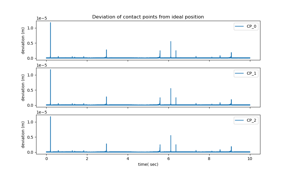
This shows, how close the contact points are to the wall. Ideally this should be zero. \(CP_X, CP_Z\) are used further down, when plotting the energies, so this must be run before the energies are run. For some reason, this takes a long time to run. In my trial runs, the errors of all \(CP_i\) were (almost?) identical, I do not know, why.
CP_X = np.empty((schritte, n))
CP_Z = np.empty((schritte, n))
for i in range(schritte):
for kk in range(n):
if (bCP_lam(*[resultat[i, j] for j in range(resultat.shape[1])],
*pL1_vals)[kk] < RW1 - r01):
CP_X[i] = CP_ort_lam(*[resultat[i, j]
for j in range(resultat.shape[1])],
*pL1_vals)[kk][0]
CP_Z[i] = CP_ort_lam(*[resultat[i, j]
for j in range(resultat.shape[1])],
*pL1_vals)[kk][1]
else:
CP_X[i] = CPh_ort_lam(*[resultat[i, j]
for j in range(resultat.shape[1])],
*pL1_vals)[kk][0]
CP_Z[i] = CPh_ort_lam(*[resultat[i, j]
for j in range(resultat.shape[1])],
*pL1_vals)[kk][1]
CPRR = []
for kk in range(n):
CPR = []
for i in range(schritte):
CPR.append(np.sqrt(np.abs(RW1**2 - CP_X[i][kk]**2 - CP_Z[i][kk]**2)))
CPRR.append(CPR)
fig, axes = plt.subplots(n, 1, sharex=True)
fig.set_size_inches((10.0, 2.0*n))
for kk in range(n):
if kk == 0:
axes[kk].set_title("Deviation of contact points from ideal position")
axes[kk].plot(times, CPRR[kk], label='CP_'+str(kk))
axes[kk].set_ylabel('deviation (m)')
if kk == n-1:
axes[kk].set_xlabel('time( sec)')
_ = axes[kk].legend()
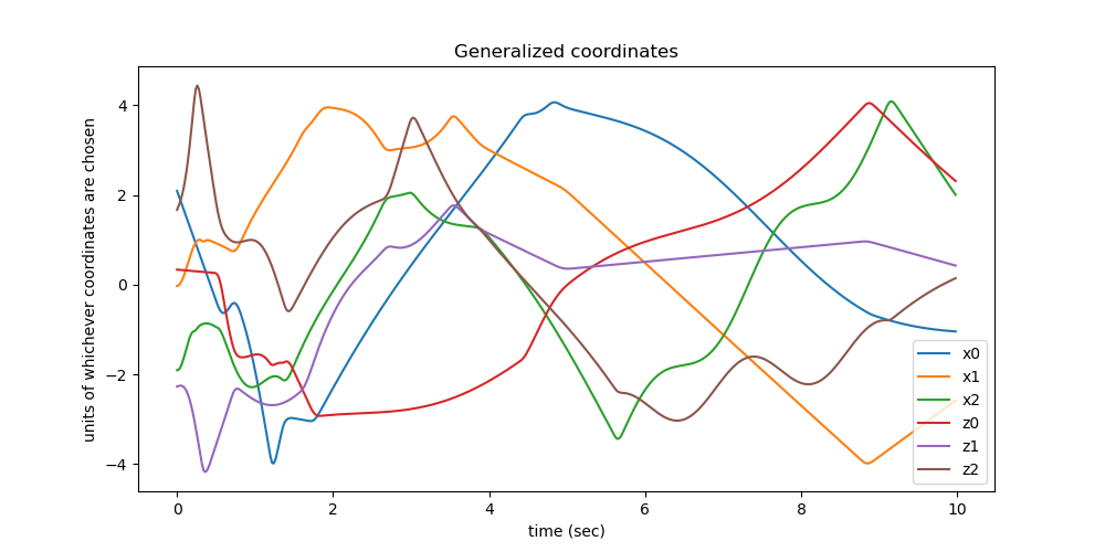
Plot whichever generalized coordinates you want to see. schritte may be very large, to catch the impacts, this is not needed her. Hence I reduce the number of points to be plotted to around \(N_2\).
N2 = 500
N1 = int(resultat.shape[0] / N2)
times1 = []
resultat1 = []
for i in range(resultat.shape[0]):
if i % N1 == 0:
times1.append(times[i])
resultat1.append(resultat[i])
resultat1 = np.array(resultat1)
times1 = np.array(times1)
bezeichnung = (['x' + str(i) for i in range(n)] +
['z' + str(i) for i in range(n)] +
['q' + str(i) for i in range(n)] +
['ux' + str(i) for i in range(n)] +
['uz' + str(i) for i in range(n)] +
['u' + str(i) for i in range(n)])
fig, ax = plt.subplots(figsize=(10, 5))
for i in range(0*n, 2*n):
label = 'gen. coord. ' + str(i)
ax.plot(times1, resultat1[:, i], label=bezeichnung[i])
ax.set_title('Generalized coordinates')
ax.set_xlabel('time (sec)')
ax.set_ylabel('units of whichever coordinates are chosen')
_ = ax.legend()
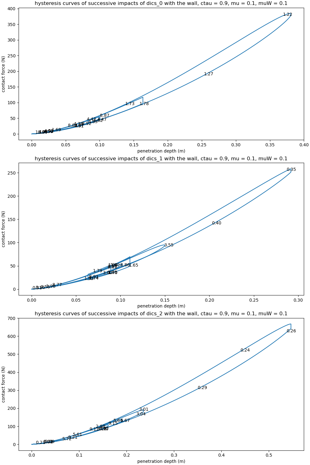
Plot the hysteresis curve of \(disc_i\) when it collides with the wall and \(disc_i\) when it collides with \(disc_j\), \(i < j\) The \(i_0\) is needed to get the (approximately) correct \(\dot \rho^{(-)}\), the speed at the impact. I only plot, if an impact did take place. The black numbers on the curves give the time of the impact.
vDmc = [Dmc_list[i].vel(N).magnitude() for i in range(n)]
vorzeichen = [sm.sign(me.dot(Dmc_list[i].pos_from(P0).normalize(),
Dmc_list[i].vel(N).normalize()))
for i in range(n)]
vDmc_lam = sm.lambdify(qL + pL2, vDmc, cse=True)
vorzeichen_lam = sm.lambdify(qL + pL2, vorzeichen, cse=True)
HC_kraft_list = []
HC_displ_list = []
HC_times_list = []
l1_list = []
for l1 in range(n):
HC_kraft = []
HC_displ = []
HC_times = []
zaehler = 0
i0 = 0
for i in range(resultat.shape[0]):
abstand = r01 - abstandDmcCP_lam(*[resultat[i, j]
for j in range(resultat.shape[1])],
*pL1_vals)[l1]
if abstand < 0.:
i0 = i+1
if abstand >= 0. and i0 == i:
walldt = vDmc_lam(*[resultat[i, j]
for j in range(resultat.shape[1])],
*pL2_vals)[l1]
if abstand >= 0.:
rhodt = (vorzeichen_lam(*[resultat[i, j]
for j in range(resultat.shape[1])],
*pL2_vals)[l1] *
vDmc_lam(*[resultat[i, j]
for j in range(resultat.shape[1])],
*pL2_vals)[l1])
kraft0 = (k0W1 * abstand**(3/2) * (1. + 3./2. * (1 - ctau1) *
rhodt/walldt))
HC_displ.append(abstand)
HC_kraft.append(kraft0)
HC_times.append((zaehler, times[i]))
zaehler += 1
if len(HC_displ) > 0:
HC_displ = np.array(HC_displ)
HC_kraft = np.array(HC_kraft)
HC_displ_list.append(HC_displ)
HC_kraft_list.append(HC_kraft)
HC_times_list.append(HC_times)
l1_list.append(l1)
fig, ax = plt.subplots(len(HC_displ_list), 1,
figsize=(10, 5.0 * len(HC_displ_list)),
layout='constrained')
for i in range(len(HC_displ_list)):
HC_displ = HC_displ_list[i]
HC_kraft = HC_kraft_list[i]
HC_times = HC_times_list[i]
ax[i].plot(HC_displ, HC_kraft)
ax[i].set_ylabel('contact force (N)')
ax[i].set_title((f'hysteresis curves of successive impacts of '
f'dics_{l1_list[i]}'
f' with the wall, ctau = {ctau1}, '
f'mu = {mu1}, muW = {muW1}'))
ax[i].set_xlabel('penetration depth (m)')
zeitpunkte = 20
reduction = max(1, int(len(HC_times)/zeitpunkte))
for k in range(len(HC_times)):
if k % reduction == 0:
coord = HC_times[k][0]
ax[i].text(HC_displ[coord], HC_kraft[coord],
f'{HC_times[k][1]:.2f}', color="black")
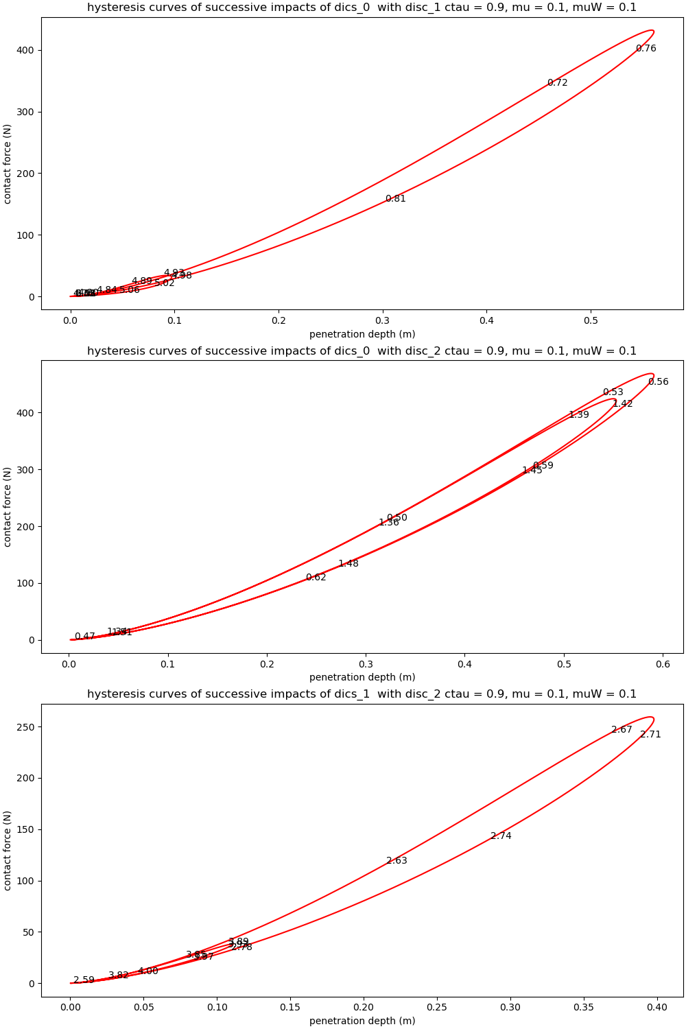
plot the hysteresis curve of disc i colliding with disc j, for i < j only,
zaehler1 = -1
HC_kraft_list = []
HC_displ_list = []
HC_times_list = []
l1_list = []
l2_list = []
for l1, l2 in permutations(range(n), r=2):
zaehler1 += 1
HC_kraft = []
HC_displ = []
HC_times = []
zaehler = 0
i0 = 0
for i in range(resultat.shape[0]):
abstand = 2.*r01 - Dmc_distanz_lam(*[resultat[i, j]
for j in range(2*n)])[zaehler1]
if abstand < 0.:
i0 = i+1
if abstand >= 0. and i0 == i:
walldt = rhomax_list_lam(*[resultat[i, j]
for j in range(resultat.shape[1])],
*pL1_vals)[zaehler1]
if abstand >= 0.:
rhodt = rhomax_list_lam(*[resultat[i, j]
for j in range(resultat.shape[1])],
*pL1_vals)[zaehler1]
kraft0 = (k01 * abstand**(3/2) * (1. + 3./2. * (1 - ctau1) *
rhodt/walldt))
HC_displ.append(abstand)
HC_kraft.append(kraft0)
HC_times.append((zaehler, times[i]))
zaehler += 1
if len(HC_displ) > 0 and l1 < l2:
HC_displ = np.array(HC_displ)
HC_kraft = np.array(HC_kraft)
HC_displ_list.append(HC_displ)
HC_kraft_list.append(HC_kraft)
HC_times_list.append(HC_times)
l1_list.append(l1)
l2_list.append(l2)
fig, ax = plt.subplots(len(HC_displ_list), 1,
figsize=(10, 5.0 * len(HC_displ_list)),
layout='constrained')
for i in range(len(HC_displ_list)):
HC_displ = HC_displ_list[i]
HC_kraft = HC_kraft_list[i]
HC_times = HC_times_list[i]
l1 = l1_list[i]
l2 = l2_list[i]
ax[i].plot(HC_displ, HC_kraft, color='red')
ax[i].set_xlabel('penetration depth (m)')
ax[i].set_ylabel('contact force (N)')
ax[i].set_title((f'hysteresis curves of successive impacts of dics_{l1} '
f' with disc_{l2}'
f' ctau = {ctau1}, mu = {mu1}, muW = {muW1}'))
zeitpunkte = 12
reduction = max(1, int(len(HC_times)/zeitpunkte))
for k in range(len(HC_times)):
if k % reduction == 0:
coord = HC_times[k][0]
ax[i].text(HC_displ[coord], HC_kraft[coord],
f'{HC_times[k][1]:.2f}', color="black")
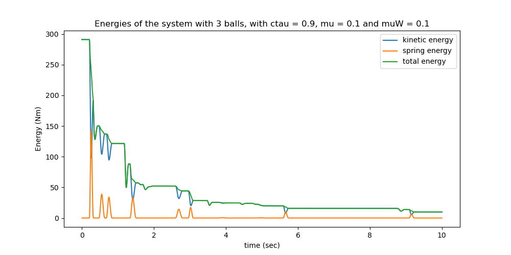
Plot the energies of the system.
If \(c_{\tau} < 1.0\), or \(m_u \neq 0\), or \(m_{uW} \neq 0\) the total energy should drop monotonically. This is due to the Hunt-Crossley prescription of the forces during a collision, due to friction during the collisions respectively. Unless the step size is very small, all impacts may not be shown. However, this would increase the running time a lot!
kin_np = np.empty(schritte)
spring_np = np.empty(schritte)
total_np = np.empty(schritte)
for i in range(schritte):
kin_np[i] = kin_lam(*[resultat[i, j] for j in range(resultat.shape[1])],
*pL2_vals)
spring_np[i] = spring_lam(*[resultat[i, j]
for j in range(resultat.shape[1])],
*pL2_vals, *[CP_X[i, j] for j in range(n)],
*[CP_Z[i, j] for j in range(n)])
total_np[i] = spring_np[i] + kin_np[i]
fig, ax = plt.subplots(figsize=(10, 5))
for i, j in zip((kin_np, spring_np, total_np),
('kinetic energy', 'spring energy', 'total energy')):
ax.plot(times, i, label=j)
ax.set_xlabel('time (sec)')
ax.set_ylabel('Energy (Nm)')
ax.set_title((f'Energies of the system with {n} balls, with ctau = {ctau1}, '
f'mu = {mu1} and muW = {muW1}'))
_ = ax.legend()
Animation
As the number of points in time, given as schritte may be verly large, I limit to around zeitpunkte. Otherwise it would take a very long time to finish the animation.
The size of the discs, and the depth of penetration is not to scale.
times2 = []
resultat2 = []
zeitpunkte = 500
reduction = max(1, int(len(times)/zeitpunkte))
for i in range(len(times)):
if i % reduction == 0:
times2.append(times[i])
resultat2.append(resultat[i])
schritte2 = len(times2)
resultat2 = np.array(resultat2)
times2 = np.array(times2)
print('number of points considered:', len(times2))
Dmc_X = np.array([[resultat2[i, j] for j in range(n)]
for i in range(schritte2)])
Dmc_Z = np.array([[resultat2[i, j] for j in range(n, 2*n)]
for i in range(schritte2)])
Po_X = np.empty((schritte2, n))
Po_Z = np.empty((schritte2, n))
CP_X = np.empty((schritte2, n))
CP_Z = np.empty((schritte2, n))
for i in range(schritte2):
Po_X[i] = [Po_pos_lam(*[resultat2[i, j] for j in range(resultat.shape[1])],
*pL2_vals)[l][0] for l in range(n)]
Po_Z[i] = [Po_pos_lam(*[resultat2[i, j] for j in range(resultat.shape[1])],
*pL2_vals)[l][1] for l in range(n)]
for i in range(schritte2):
for kk in range(n):
if (bCP_lam(*[resultat2[i, j] for j in range(resultat2.shape[1])],
*pL1_vals)[kk] < RW1 - r01):
CP_X[i] = CP_ort_lam(*[resultat2[i, j]
for j in range(resultat.shape[1])],
*pL1_vals)[kk][0]
CP_Z[i] = CP_ort_lam(*[resultat2[i, j]
for j in range(resultat.shape[1])],
*pL1_vals)[kk][1]
else:
CP_X[i] = CPh_ort_lam(*[resultat2[i, j]
for j in range(resultat.shape[1])],
*pL1_vals)[kk][0]
CP_Z[i] = CPh_ort_lam(*[resultat2[i, j]
for j in range(resultat.shape[1])],
*pL1_vals)[kk][1]
# This is to asign colors of 'plasma' to the discs.
Test = mp.colors.Normalize(0, n)
Farbe = mp.cm.ScalarMappable(Test, cmap='plasma')
farben = [Farbe.to_rgba(l) for l in range(n)] # color of starting position
def animate_pendulum(times2, Dmc_x, Dmc_Z, Po_X, Po_Z):
fig, ax = plt.subplots(figsize=(8, 8))
ax.axis('on')
theta = np.linspace(0., 2.*np.pi, 200)
aa = RW1 * np.sin(theta)
bb = RW1 * np.cos(theta)
ax.plot(aa, bb, linewidth=2)
LINE1 = []
LINE2 = []
LINE3 = []
for i in range(n):
# picking the 'right' radius of the discs I do by trial and error.
line1, = ax.plot([], [], 'o', markersize=400./RW1)
line2, = ax.plot([], [], 'o', markersize=5, color='black')
line3, = ax.plot([], [], '-', markersize=0, linewidth=0.3)
LINE1.append(line1)
LINE2.append(line2)
LINE3.append(line3)
def animate(i):
ax.set_title((f'System with {n} bodies, running time'
f'{i/schritte2 * intervall:.2f} sec \n '
f'ctau = {ctau1}, mu = {mu1}, muW = {muW1}'),
fontsize=12)
for j in range(n):
LINE1[j].set_data([Dmc_X[i, j]], [Dmc_Z[i, j]])
LINE1[j].set_color(farben[j])
LINE2[j].set_data([Po_X[i, j]], [Po_Z[i, j]])
LINE3[j].set_data([Dmc_X[:i, j]], [Dmc_Z[:i, j]])
LINE3[j].set_color(farben[j])
return LINE1 + LINE2 + LINE3
anim = animation.FuncAnimation(fig, animate, frames=schritte2,
interval=1000*times2.max() / schritte2,
blit=True)
return anim
anim = animate_pendulum(times2, Dmc_X, Dmc_Z, Po_X, Po_Z)
plt.show()