Spacecraft with Nutation Damper

Objectives

• Show how to model a spacecraft with a nutation damper.

• Show how to optimize the dampening.

Description

A spacecraft in empty space, no gravitation, is equipped with a nutation damper. It is described in Dynamics. Theory and Application of Kane's Method by Carlos M. Roithmay and Dewey H Hodges, Section 9.6.

It is also described here: https://nescacademy.nasa.gov/video/37db5926a05747bea43a7a7c82663bc11d

Notes

• One must not forget to add the reaction force / torque on \(B_O\), the center of mass of the spacecraft.

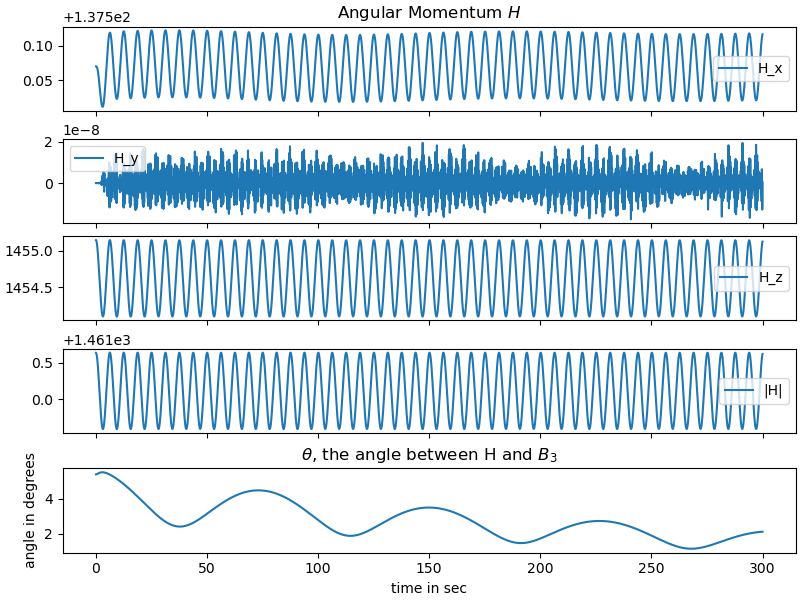
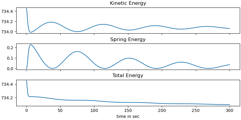
• As there are no external torques / forces the angular momentum is conserved, while the total energy drops, due to the friction in the system.

• The labelling of the axes of the body frame B follows the NASA lecture given above. \(q_4\) is called \(z\) in that lecture; \(\dfrac{d}{dt}z\) there is called \(u_4\) here.

States

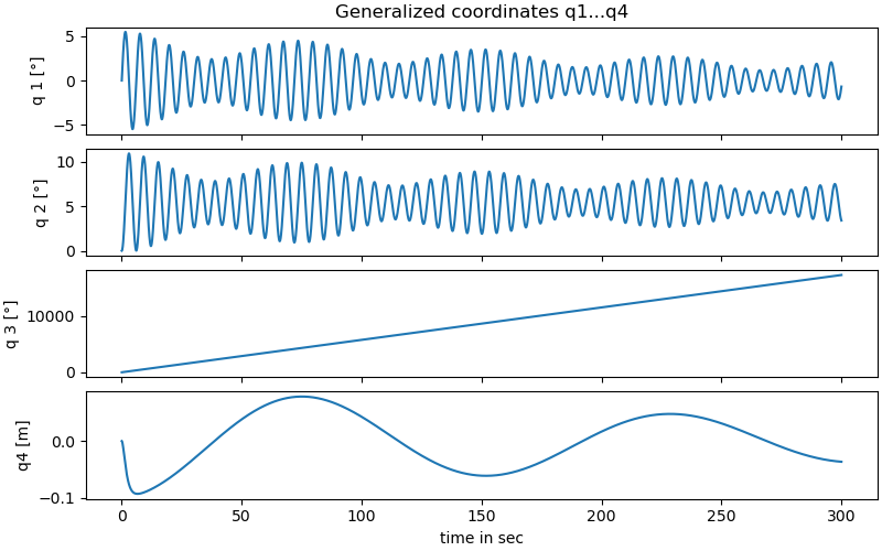
• \(q_1, q_2, q_3\) : The Euler angles of the rotation of the spacecraft w.r.t. the inertial frame N.

• \(q_4\) : The displacement of the nutation damper in the B.z-direction.

• \(q_5, q_6, q_7\) : The position coordinates of the center of mass of the spacecraft.

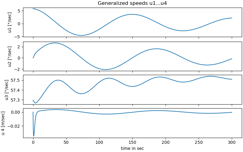
• \(u_1, u_2, u_3\) : The angular velocities of the spacecraft.

• \(u_4\) : The velocity of the nutation damper in the B.z-direction.

• \(u_5, u_6, u_7\) : The velocities of the center of mass of the spacecraft.

Parameters

• \(e\) : The distance from the center of mass of the spacecraft to the particle P.

• \(k\) : The stiffness of the nutation damper, to be optimized later

• \(c\) : The damping coefficient of the nutation damper, to be optimized later

• \(I_1\) : The moment of inertia of the spacecraft about the B.x-axis.

• \(I_2\) : The moment of inertia of the spacecraft about the B.y axis.

• \(I_3\) : The moment of inertia of the spacecraft around the B.z axis.

• \(m_B\) : The mass of the spacecraft.

• \(m_P\) : The mass of the particle P

• \(N\) : Inertial frame

• \(B\) : Body frame of the spacecraft

• \(B_O\) : mass center of the body of the spacecraft

• \(\theta\) : The angle between the B.z axis and the (constant) vector of the angular momentum. Not really a parameter, but the quantity of maximum interest here.

import sympy as sm
import numpy as np
import matplotlib.pyplot as plt
import sympy.physics.mechanics as me
from scipy.integrate import solve_ivp
from scipy.interpolate import CubicSpline
from scipy.optimize import root

from mpl_toolkits.mplot3d.art3d import Poly3DCollection
from matplotlib.animation import FuncAnimation

from opty import Problem

Set Up Kane’s Equations of Motion

# Reference Frames
N, B = me.ReferenceFrame('N'), me.ReferenceFrame('B')
# Points
O, BO, P = me.Point('O'), me.Point('BO'), me.Point('P')
O.set_vel(N, 0)
t = me.dynamicsymbols._t

# Generalized coordinates and speeds
q1, q2, q3, q4, q5, q6, q7 = me.dynamicsymbols('q_1 q_2 q_3 q_4 q_5 q_6 q_7')
u1, u2, u3, u4, u5, u6, u7 = me.dynamicsymbols('u_1 u_2 u_3 u_4 u_5 u_6 u_7')

I1, I2, I3, mB, mP, k, c, e = sm.symbols('I_1, I_2, I_3, m_B, m_P, k, c, e')

# Describe the system
B.orient_body_fixed(N, (q1, q2, q3), '123')
rot = B.ang_vel_in(N)
B.set_ang_vel(N, u1 * B.x + u2 * B.y + u3 * B.z)
rot1 = B.ang_vel_in(N)

BO.set_pos(O, q5 * N.x + q6 * N.y + q7 * N.z)
BO.set_vel(N, u5 * N.x + u6 * N.y + u7 * N.z)

P.set_pos(BO, e * B.x + q4 * B.z)
P.set_vel(B, u4 * B.z)

# Create the bodies
inertiaB = me.inertia(B, I1, I2, I3)
bodyB = me.RigidBody('bodyB', BO, B, mB, (inertiaB, BO))
bodyP = me.Particle('bodyP', P, mP)
bodies = [bodyB, bodyP]

# Forces, reaction force and couple
forces = [
    (P, -(k * q4 + c * u4) * B.z),
    (BO, (k * q4 + c * u4) * B.z),
    (B, (e * B.x).cross(((k * q4 + c * u4) * B.z)))
]

# Kinematic equations.
kd = sm.Matrix([
    *[(rot - rot1).dot(uv) for uv in N],
    u4 - q4.diff(t),
    u5 - q5.diff(t),
    u6 - q6.diff(t),
    u7 - q7.diff(t),
])

This dictionary is needed to replace the derivatives in the angular momentum further down.

solution = sm.solve(kd, (q1.diff(t), q2.diff(t), q3.diff(t),
                         q4.diff(t), q5.diff(t), q6.diff(t), q7.diff(t)))
for i in solution.keys():
    print(f"{i} = {solution[i]}")

Derivative(q_1(t), t) = u_1(t)*cos(q_3(t))/(sin(q_3(t))**2*cos(q_2(t)) + cos(q_2(t))*cos(q_3(t))**2) - u_2(t)*sin(q_3(t))/(sin(q_3(t))**2*cos(q_2(t)) + cos(q_2(t))*cos(q_3(t))**2)
Derivative(q_2(t), t) = u_1(t)*sin(q_3(t))/(sin(q_3(t))**2 + cos(q_3(t))**2) + u_2(t)*cos(q_3(t))/(sin(q_3(t))**2 + cos(q_3(t))**2)
Derivative(q_3(t), t) = -u_1(t)*sin(q_2(t))*cos(q_3(t))/(sin(q_3(t))**2*cos(q_2(t)) + cos(q_2(t))*cos(q_3(t))**2) + u_2(t)*sin(q_2(t))*sin(q_3(t))/(sin(q_3(t))**2*cos(q_2(t)) + cos(q_2(t))*cos(q_3(t))**2) + u_3(t)*sin(q_3(t))**2*cos(q_2(t))/(sin(q_3(t))**2*cos(q_2(t)) + cos(q_2(t))*cos(q_3(t))**2) + u_3(t)*cos(q_2(t))*cos(q_3(t))**2/(sin(q_3(t))**2*cos(q_2(t)) + cos(q_2(t))*cos(q_3(t))**2)
Derivative(q_4(t), t) = u_4(t)
Derivative(q_5(t), t) = u_5(t)
Derivative(q_6(t), t) = u_6(t)
Derivative(q_7(t), t) = u_7(t)

Kanes equations

q_ind = [q1, q2, q3, q4, q5, q6, q7]
u_ind = [u1, u2, u3, u4, u5, u6, u7]

kane = me.KanesMethod(N, q_ind=q_ind, u_ind=u_ind, kd_eqs=kd)
fr, frstar = kane.kanes_equations(bodies, forces)
for i in range(fr.shape[0]):
    fr[i] = fr[i].simplify()
    frstar[i] = frstar[i].simplify()

MM = kane.mass_matrix_full
force = kane.forcing_full

H = me.angular_momentum(BO, N, *bodies).subs(solution)
theta = sm.acos((H.normalize()).dot(B.z))

Hx = H.dot(N.x)
Hy = H.dot(N.y)
Hz = H.dot(N.z)

kin_energie = sum(me.kinetic_energy(N, b).subs({q4.diff(t): u4})
                  for b in bodies)
spring_energie = 0.5 * k * q4**2

qL = q_ind + u_ind
pL = [mB, mP, I1, I2, I3, k, c, e]

Convert sympy functions to numpy functions

MM_lam = sm.lambdify(qL + pL, MM, cse=True)
force_lam = sm.lambdify(qL + pL, force, cse=True)
H_lam = sm.lambdify(qL + pL, [Hx, Hy, Hz], cse=True)
H_abs_lam = sm.lambdify(qL + pL, H.magnitude(), cse=True)
kin_lam = sm.lambdify(qL + pL, kin_energie, cse=True)
spring_lam = sm.lambdify(qL + pL, spring_energie, cse=True)

theta_lam = sm.lambdify(qL + pL, theta, cse=True)

Numerical integration

# Input variables
I11 = 1375.7
I21 = 1292.5
I31 = 1402.4
mB1 = 5274.4
mP1 = 52.744
e1 = 1.0
k1 = 52.744
c1 = 105.49

u11 = 0.1
u21 = 0.0
u31 = 1.0
u41 = 0.0
u51 = 0.0
u61 = 0.0
u71 = 0.0

q11 = 0.0
q21 = 0.0
q31 = 0.0
q41 = 0.0
q51 = 0.0
q61 = 0.0
q71 = 0.0

intervall = 300.0
punkte = 10.0

# Needed for plotting, below
k1b = k1
c1b = c1

schritte = int(intervall * punkte)
times = np.linspace(0., intervall, schritte)
t_span = (0., intervall)

pL_vals = [mB1, mP1, I11, I21, I31, k1, c1, e1]
y0 = [q11, q21, q31, q41, q51, q61, q71, u11, u21, u31, u41, u51, u61, u71]


def gradient(t, y, args):
    sol = np.linalg.solve(MM_lam(*y, *args), force_lam(*y, *args))
    return np.array(sol).T[0]


resultat1 = solve_ivp(gradient, t_span, y0, t_eval=times, args=(pL_vals,),
                      atol=1.e-12, rtol=1.e-12,
                      )

resultat_int = resultat1.y.T
print('resultat shape', resultat_int.shape, '\n')
print(resultat1.message, '\n')

print(f"To numerically integrate an intervall of {intervall} sec "
      f"the routine cycled {resultat1.nfev} times")

resultat shape (3000, 14)

The solver successfully reached the end of the integration interval.

To numerically integrate an intervall of 300.0 sec the routine cycled 24950 times

Print Angular Momentum and angle theta

H_values = H_lam(*[resultat_int[:, i] for i in
                   range(resultat_int.shape[1])], *pL_vals)

fig, ax = plt.subplots(5, 1, figsize=(8, 6), layout='constrained',
                       sharex=True)
ax[0].plot(times, H_values[0], label='H_x')
ax[1].plot(times, H_values[1], label='H_y')
ax[2].plot(times, H_values[2], label='H_z')
ax[4].plot(times, np.rad2deg(theta_lam(*[resultat_int[:, i] for i in
                             range(resultat_int.shape[1])], *pL_vals)))
ax[4].set_title(f"$\\theta$, the angle between H and $B_3$")
ax[4].set_ylabel('angle in degrees')
ax[3].plot(times, H_abs_lam(*[resultat_int[:, i] for i in
                              range(resultat_int.shape[1])], *pL_vals),
           label='|H|')

[a.legend() for a in [ax[j] for j in range(4)]]
ax[-1].set_xlabel('time in sec')
_ = ax[0].set_title('Angular Momentum $H$')

plot results q1…q4

fig, ax = plt.subplots(4, 1, figsize=(8, 5), layout='constrained',
                       sharex=True)
ax[0].set_title('Generalized coordinates q1...q4')
ax[-1].set_xlabel('time in sec')
for i in range(4):
    if i < 3:
        ax[i].plot(times, np.rad2deg(resultat_int[:, i]))
        ax[i].set_ylabel(f'q {i+1} [°]')
    else:
        ax[i].plot(times, resultat_int[:, i])
        ax[i].set_ylabel(f'q{i+1} [m]')

plot results u1…u4

fig, ax = plt.subplots(4, 1, figsize=(8, 5), layout='constrained',
                       sharex=True)
ax[0].set_title('Generalized speeds u1...u4')
ax[-1].set_xlabel('time in sec')
for j in range(4):
    if j < 3:
        ax[j].plot(times, np.rad2deg(resultat_int[:, j+7]))
        ax[j].set_ylabel(f'u{j+1} [°/sec]')
    else:
        ax[j].plot(times, resultat_int[:, j+7])
        ax[j].set_ylabel(f'u {j+1} [m/sec]')

Plot the energies

fig, ax = plt.subplots(3, 1, figsize=(8, 4), sharex=True, layout='constrained')
ax[0].plot(times, kin_lam(*[resultat_int[:, i] for i in
                          range(resultat_int.shape[1])], *pL_vals))
ax[0].set_title('Kinetic Energy')
ax[1].plot(times, spring_lam(*[resultat_int[:, i] for i in
                               range(resultat_int.shape[1])], *pL_vals))
ax[1].set_title('Spring Energy')
ax[2].plot(times, kin_lam(*[resultat_int[:, i] for i in
                            range(resultat_int.shape[1])], *pL_vals) +
           spring_lam(*[resultat_int[:, i] for i in
                        range(resultat_int.shape[1])], *pL_vals))
ax[2].set_title('Total Energy')
ax[-1].set_xlabel('time in sec')

# Set Up the Optimization and Solve It
# ------------------------------------

# Set up equations of motion suitable for opty.
EOM_opty = kd.col_join(fr + frstar)

state_symbols = q_ind + u_ind
t0, tf = 0.0, intervall
num_nodes = int(intervall * punkte)
interval_value = (tf - t0) / num_nodes

par_map = {}
par_map[mB] = mB1
par_map[mP] = mP1
par_map[I1] = I11
par_map[I2] = I21
par_map[I3] = I31
par_map[e] = e1

instance_constraints = (
    (q1.func(t0) - q11),
    (q2.func(t0) - q21),
    (q3.func(t0) - q31),
    (q4.func(t0) - q41),
    (q5.func(t0) - q51),
    (q6.func(t0) - q61),
    (q7.func(t0) - q71),
    (u1.func(t0) - u11),
    (u2.func(t0) - u21),
    (u3.func(t0) - u31),
    (u4.func(t0) - u41),
    (u5.func(t0) - u51),
    (u6.func(t0) - u61),
    (u7.func(t0) - u71),
)

# Bounds for, say, physical or geometric reasons.
bounds = {
    k: (0.0, 200),
    c: (0.0, 500),
    q4: (-1.0, 1.0)
}


def obj(free):
    # Minimize the rotations around B.x and B.y
    summe = np.sum(free[7 * num_nodes: 9*num_nodes]**2)
    return summe


def obj_grad(free):
    # Gradient of the objective function
    grad = np.zeros_like(free)
    grad[7 * num_nodes: 9*num_nodes] = 2 * free[7 * num_nodes: 9*num_nodes]
    return grad


prob = Problem(
    obj,
    obj_grad,
    EOM_opty,
    state_symbols,
    num_nodes,
    interval_value,
    known_parameter_map=par_map,
    instance_constraints=instance_constraints,
    bounds=bounds,
    time_symbol=t,
)

initial_guess = np.concatenate(((resultat_int.T).flatten(),
                                np.array([100.0, 50.0])))

for _ in range(1):
    solution, info = prob.solve(initial_guess)
    initial_guess = solution
    print(info['status_msg'])
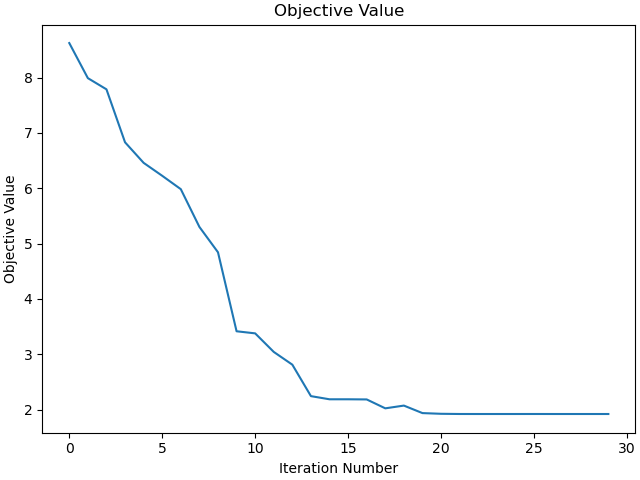
    print(f"Objective value: {info['obj_val']:.2f}")

b'Algorithm terminated successfully at a locally optimal point, satisfying the convergence tolerances (can be specified by options).'
Objective value: 1.92

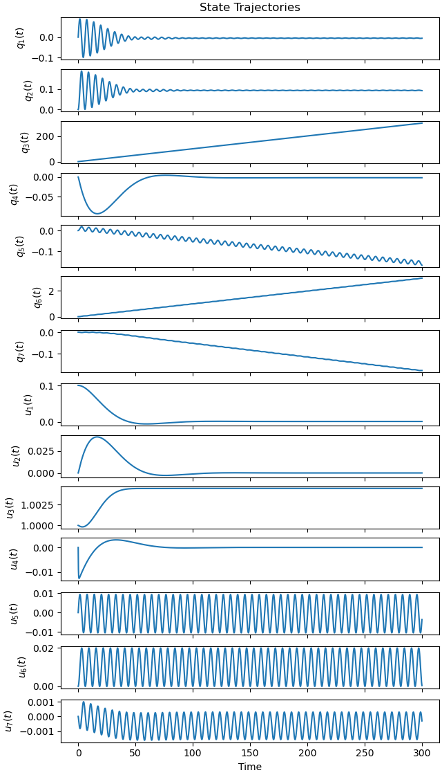
Plot the results

_ = prob.plot_trajectories(solution)

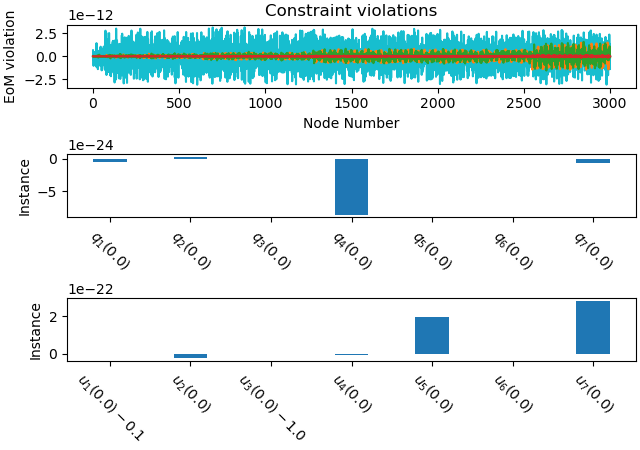
Plot the errors

_ = prob.plot_constraint_violations(solution)

Plot the objective value

_ = prob.plot_objective_value()
print('Sequence of unknown parameters:', prob.collocator.unknown_parameters)
print(f"c: {solution[-2]:.2f}")
print(f"k: {solution[-1]:.2f}")

Sequence of unknown parameters: (c, k)
c: 367.41
k: 34.77

state_sol, *_ = prob.parse_free(solution)
resultat = state_sol.T
c1 = solution[-2]
k1 = solution[-1]

get the dimensions of the body. Only needed to get an idea hwo to draw the body B.

def get_dimensions(x):
    """
    Get the dimensions of a solid brick of mass mB and
    principal moments of inertia I1, I2, I3.
    """
    a, b, c = x

    return [
        I11 - 1.0 / 12.0 * mB1 * (b**2 + c**2),
        I21 - 1.0 / 12.0 * mB1 * (a**2 + c**2),
        I31 - 1.0 / 12.0 * mB1 * (a**2 + b**2)
    ]


x0 = (10.0, 10.0, 10.0)
for _ in range(2):
    loesung = root(get_dimensions, x0)
    x0 = loesung.x
    loesung = root(get_dimensions, x0)
    x0 = loesung.x
print('side lengths in m:', loesung.x)
print('Accuracy:', loesung.fun)

side lengths in m: [1.22502349 1.29999008 1.19997346]
Accuracy: [2.27373675e-13 2.27373675e-13 0.00000000e+00]

Animation

# Due to storage reason, the video is shorted to the first around 55 sec of
# the simulation.
factor = 55 / intervall
resultat_kurz = np.array((resultat[0: int(resultat.shape[0] * factor), :]))
print('resultat_kurz shape', resultat_kurz.shape)
ende = times[resultat_kurz.shape[0]]
times1 = times[0: resultat_kurz.shape[0]]
t_arr = np.linspace(0.0, ende, resultat_kurz.shape[0])

fps = 1.5
state_sol = CubicSpline(t_arr, resultat_kurz, axis=0)

# Rotation matrix functions


def rotation_matrix_x(theta):
    return np.array([
        [1, 0, 0],
        [0, np.cos(theta), -np.sin(theta)],
        [0, np.sin(theta), np.cos(theta)]
    ])


def rotation_matrix_y(theta):
    return np.array([
        [np.cos(theta), 0, np.sin(theta)],
        [0, 1, 0],
        [-np.sin(theta), 0, np.cos(theta)]
    ])


def rotation_matrix_z(theta):
    return np.array([
        [np.cos(theta), -np.sin(theta), 0],
        [np.sin(theta), np.cos(theta), 0],
        [0, 0, 1]
    ])


# Create a brick's corner points (centered at origin)
lx, ly, lz = loesung.x
brick_points = np.array([
    [-lx/2, -ly/2, -lz/2],
    [lx/2, -ly/2, -lz/2],
    [lx/2,  ly/2, -lz/2],
    [-lx/2,  ly/2, -lz/2],
    [-lx/2, -ly/2,  lz/2],
    [lx/2, -ly/2,  lz/2],
    [lx/2,  ly/2,  lz/2],
    [-lx/2,  ly/2,  lz/2]
])

# Define brick faces
faces_idx = [
    [0, 1, 2, 3],  # bottom face
    [4, 5, 6, 7],  # top face
    [0, 1, 5, 4],  # front face
    [2, 3, 7, 6],  # back face
    [1, 2, 6, 5],  # right face
    [0, 3, 7, 4]   # left face
]

# Plot setup
fig = plt.figure(figsize=(10, 10))
ax = fig.add_subplot(111, projection='3d')

pfeil = max(lx, ly, lz)
total_min = np.min(resultat[:, 4:7])
total_max = np.max(resultat[:, 4:7])
ax.set_xlim(total_min - pfeil, total_max + pfeil)
ax.set_ylim(total_min - pfeil, total_max + pfeil)
ax.set_zlim(total_min - pfeil, total_max + pfeil)
ax.set_aspect('equal')
ax.scatter([0], [0], [0], color='black', s=50)  # origin point

ax.set_xlabel(f'Inertial axis $N_1$')
ax.set_ylabel(f'Inertial axis $N_2$')
ax.set_zlabel(f'Inertial axis $N_3$')


poly = Poly3DCollection([], alpha=0.5, facecolor='cyan', edgecolor='black')
ax.add_collection3d(poly)

# Define the points in the body-fixed frame, and the head of the angular
# momentum
length = sm.sqrt(Hx**2 + Hy**2 + Hz**2)
Hx = Hx / length
Hy = Hy / length
Hz = Hz / length

P_x, P_y, P_z, H_head = sm.symbols('P_x P_y P_z H_head', cls=me.Point)
P_x.set_pos(BO, 2 * pfeil * B.x)
P_y.set_pos(BO, 2 * pfeil * B.y)
P_z.set_pos(BO, 2 * pfeil * B.z)
H_head.set_pos(BO, 4.0 * (Hx * N.x + Hy * N.y + Hz * N.z))

coordinates = BO.pos_from(O).to_matrix(N)
for point in (P_x, P_y, P_z, H_head):
    coordinates = coordinates.row_join(point.pos_from(O).to_matrix(N))

coords_lam = sm.lambdify(qL + pL, coordinates, cse=True)

x_axis = ax.quiver(0, 0, 0, 0, 0, 0, color='red', arrow_length_ratio=0.1)
y_axis = ax.quiver(0, 0, 0, 0, 0, 0, color='blue', arrow_length_ratio=0.1)
z_axis = ax.quiver(0, 0, 0, 0, 0, 0, color='green', arrow_length_ratio=0.1)
ang_mom = ax.quiver(0, 0, 0, 0, 0, 0, color='purple', arrow_length_ratio=0.1)
point_BO = ax.scatter([0], [0], [0], color='black', s=50)
ax.text(
    -0.5, 2.5, -0.5,
    f"Parameters:\n"
    f"$I_{1}$ = {I11:,}\n"
    f"$I_{2}$ = {I21:,}\n"
    f"$I_{3}$ = {I31:,}\n"
    f"$m_B$ = {mB1:,}\n"
    f"$m_P$ = {mP1:,}\n"
    f"$e$ = {e1:.3f}\n"
    f"$k$ = {k1:.3f}\n"
    f"$c$ = {c1:.3f}\n",
    fontsize=12,
)

# Animation update


def update(frame):
    global x_axis, y_axis, z_axis, ang_mom
    # Rotation
    alpha = state_sol(frame)[0]
    beta = state_sol(frame)[1]
    gamma = state_sol(frame)[2]
    R = (rotation_matrix_x(alpha) @ rotation_matrix_y(beta) @
         rotation_matrix_z(gamma))
    rotated = brick_points @ R.T

    # Translation (center moving in a circle)
    center = np.array([state_sol(frame)[4], state_sol(frame)[5],
                       state_sol(frame)[6]])
    moved = rotated + center

    # Update faces
    poly.set_verts([[moved[i] for i in face] for face in faces_idx])

    # Update body fixed axes
    coords = coords_lam(*state_sol(frame), *pL_vals)
    x_axis.remove()
    y_axis.remove()
    z_axis.remove()
    ang_mom.remove()

    x_axis = ax.quiver(coords[0, 0], coords[1, 0], coords[2, 0],
                       coords[0, 1] - coords[0, 0],
                       coords[1, 1] - coords[1, 0],
                       coords[2, 1] - coords[2, 0],
                       color='red', arrow_length_ratio=0.1)

    y_axis = ax.quiver(coords[0, 0], coords[1, 0], coords[2, 0],
                       coords[0, 2] - coords[0, 0],
                       coords[1, 2] - coords[1, 0],
                       coords[2, 2] - coords[2, 0],
                       color='blue', arrow_length_ratio=0.1)

    z_axis = ax.quiver(coords[0, 0], coords[1, 0], coords[2, 0],
                       coords[0, 3] - coords[0, 0],
                       coords[1, 3] - coords[1, 0],
                       coords[2, 3] - coords[2, 0],
                       color='green', arrow_length_ratio=0.1)

    ang_mom = ax.quiver(coords[0, 0], coords[1, 0], coords[2, 0],
                        coords[0, 4] - coords[0, 0],
                        coords[1, 4] - coords[1, 0],
                        coords[2, 4] - coords[2, 0],
                        color='purple', arrow_length_ratio=0.1)

    ax.set_title(f"Example of David Levinson's lecture No 6 \n "
                 f"Running time: {frame:.2f} sec / High speed video \n "
                 f"Red arrow is $B_1$, blue arrow is $B_2$, "
                 f"green arrow is $B_3$ \n"
                 f"Purple arrow is the angular momentum vector $H$")

    point_BO._offsets3d = ([coords[0, 0]], [coords[1, 0]], [coords[2, 0]])

    return poly, x_axis, y_axis, z_axis, point_BO, ang_mom


ani = FuncAnimation(fig, update, frames=np.arange(0, intervall * factor,
                                                  1 / fps),
                    interval=150 / fps, blit=True)
plt.show()

Once Loop Reflect

resultat_kurz shape (550, 14)
WARNING:matplotlib.animation:MovieWriter ffmpeg unavailable; using Pillow instead.

Compare theta before / after optimization

fig, ax = plt.subplots(2, 1, figsize=(8, 3), layout='constrained',
                       sharex=True)
ax[0].plot(times, np.rad2deg(theta_lam(*[resultat_int[:, i] for i in
                                         range(resultat_int.shape[1])],
                                       *pL_vals)))
ax[0].set_title(f"$\\theta$ before optimization, \n k  = {k1b:.3f} \n "
                f"c  = {c1b:.3f}")
ax[0].set_ylabel('angle [deg]')
ax[1].plot(times, np.rad2deg(theta_lam(*[resultat[:, i] for i in
                                         range(resultat.shape[1])], *pL_vals)))
ax[1].set_title(f"$\\theta$ after optimization, \n k  = {k1:.3f} \n "
                f"c  = {c1:.3f}")
_ = ax[1].set_ylabel('angle [deg]')