Tumor Antigionesis (betts_10_141)

This is example 10.141 from John T. Betts, Practical Methods for Optimal Control Using NonlinearProgramming, 3rd edition, Chapter 10: Test Problems. It is described in more detail in section 8.17 of the book.

Notes

• The variable \(\textrm{hilfs}\) ist itroduced to eneforce \(y(tf) \leq A\) as an instance inequality constraint, which opty presently does not support. (of course, looking at the equations of motion, it is clear that \(\dfrac{d}{dt}y(t) \geq 0\), so bounding y(t) would have been sufficient - which opty does support)

• Unless \(\left[ \textrm{num}_{\textrm{nodes}} - 1 \right] \cdot h_{\textrm{fast}}\) is chosen only a bit larger than the result, convergence becomes difficult. (trial and error approach)

States

• \(p, q, y\) : state variables

Controls

• \(u\) : control variable

import numpy as np
import sympy as sm
import sympy.physics.mechanics as me
import time
from opty import Problem
from opty.utils import MathJaxRepr

Equations of Motion

t = me.dynamicsymbols._t

p, q, y = me.dynamicsymbols('p, q, y')
u = me.dynamicsymbols('u')
hilfs = me.dynamicsymbols('hilfs')

h_fast = sm.symbols('h_fast')

Parameters

chi = 0.084
G = 0.15
b = 5.85
nu = 0.02
d = 0.00873
a = 75.0
A = 15.0

pbar = ((b - nu)/d)**(3/2)
qbar = pbar
p0 = pbar/2.0
q0 = qbar/4.0

Equations of motion.

eom = sm.Matrix([
    -p.diff(t) - chi*p*sm.ln(p/q),
    -q.diff(t) + q*(b - (nu + d*p**(2/3) + G*u)),
    -y.diff(t) + u,
    hilfs * A - y
])

MathJaxRepr(eom)

$$\left[\begin{matrix}- 0.084 p \log{\left(\frac{p}{q} \right)} - \dot{p}\\\left(- 0.00873 p^{0.666666666666667} - 0.15 u + 5.83\right) q - \dot{q}\\u - \dot{y}\\15.0 hilfs - y\end{matrix}\right]$$

Define and Solve the Optimization Problem.

num_nodes = 501

interval_value = h_fast
t0, tf = 0*h_fast, (num_nodes-1)*h_fast

state_symbols = (p, q, y)

Specify the objective function and form the gradient.

def obj(free):
    return free[num_nodes-1]


def obj_grad(free):
    grad = np.zeros_like(free)
    grad[num_nodes-1] = 1.0
    return grad

Define the instance constraints, bounds, and eom bounds.

instance_constraints = (
    p.func(t0) - p0,
    q.func(t0) - q0,
    y.func(t0),
    hilfs.func(tf) - 1.0,
)

bounds = {
    h_fast: (0.0, 2.5 / (num_nodes-1)),
    p: (0.01, pbar),
    q: (0.01, qbar),
    y: (0.0, np.inf),
    u: (0, a),
}

eom_bounds = {3: (0.0, np.inf)}

Set up the Problem.

prob = Problem(
    obj,
    obj_grad,
    eom,
    state_symbols,
    num_nodes,
    interval_value,
    instance_constraints=instance_constraints,
    bounds=bounds,
    eom_bounds=eom_bounds,
    time_symbol=t
)

Give some rough estimates for the trajectories.

initial_guess = np.ones(prob.num_free)

Find the optimal solution.

start = time.time()
solution, info = prob.solve(initial_guess)
print(f"Solved in {time.time() - start:.2f} seconds.")

Solved in 29.24 seconds.

Print some information about the solution.

print(info['status_msg'])
tfstar = 1.1961336
print(f"Duration is: {solution[-1]*(num_nodes-1):.4f} "
      f"as per the book it is {tfstar:.3f}, so the deviation is: "
      f"{(solution[-1]*(num_nodes-1) - tfstar)/tfstar*100:.3f} %")
Jstar = 7571.6712
print(f"p(tf) = {solution[num_nodes-1]:.4f}" +
      f"as per the book it is {Jstar:.4f}, so the deviation is: " +
      f"{(solution[num_nodes-1] - Jstar)/Jstar*100:.3f} %")

b'Algorithm terminated successfully at a locally optimal point, satisfying the convergence tolerances (can be specified by options).'
Duration is: 1.1788 as per the book it is 1.196, so the deviation is: -1.450 %
p(tf) = 7586.6171as per the book it is 7571.6712, so the deviation is: 0.197 %

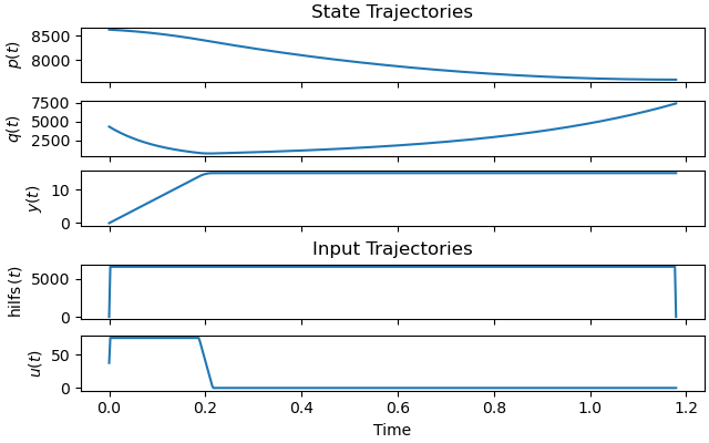
Plot the optimal state and input trajectories.

_ = prob.plot_trajectories(solution)

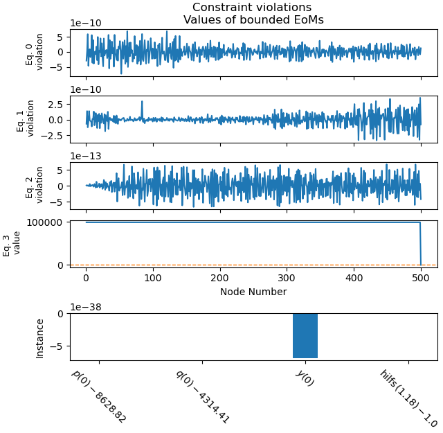
Plot the constraint violations.

_ = prob.plot_constraint_violations(solution, subplots=True, show_bounds=True)

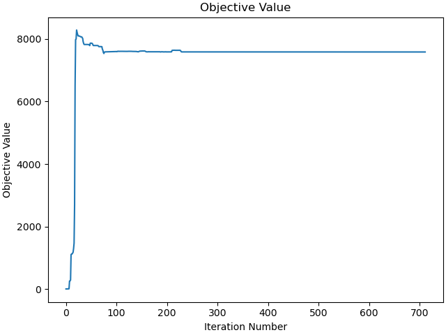
Plot the objective function as a function of optimizer iteration.

_ = prob.plot_objective_value()

sphinx_gallery_thumbnail_number = 2