Block Sliding on a Spinning Disc

Objective

• Try to simulate a very simple example of Coulomb Friction.

  https://www.youtube.com/watch?v=jaMVdTaPxgQ

Description

A disc is spinning in the horizontal X/Y plane, starting at zero angular velocity, increasing linearly with time.

A block, modeled as a particle is on the disc at a distance from the center of the disc. As the disc starts to rotate, the block initially is at rest w.r.t. the disc, but eventually the centrifugal force will overcome the static friction force, and the block will start to slide on the disc.

The resting phase is modeled that the block is tied to its starting position by a spring, which is active while the speed of the block relative to the disc is (close to) zero.

When | \({}^Av^P\) | > cut_off the spring is deactivated, and the block is subject to ( a portion of the) friction force, which the disc exerts on the block. The other portion of the friction force is due to the block moving relative to the disc and tries to slow it down.

Notes

• Changing cut_off from \(10^{-3}\) to \(10^{-4}\) increases the function calls of solve_ivp by over a factor of 50, without affecting the result much, at least visually. Further changing from \(10^{-4}\) to \(10^{-8}\) changes the number of function calls only by a factor on 1.5. No explanation.

• Using the method ‘Radau’ for the integration of the equations of motion gives completely useless results, same with BDF.

• The method ‘DOP853’ works fine but going from cut_off = \(10^{-3}\) to cut_off = \(10^{-4}\) increases the function calls of solve_ivp by over a factor of over 200.

  All this seems to indicate that this is a numerically tricky problem.

• At least qualitatively the simulation looks like the video above.

States:

• \(x\) - position of the block in the disc frame

• \(y\) - position of the block in the disc frame

• \(u_x\) - velocity of the block in the disc frame

• \(u_y\) - velocity of the block in the disc frame

Parameters:

• \(m\) - mass of the block

• \(g\) - gravitational acceleration

• \(\omega\) - angular velocity of the disc

• \(\mu_{\textrm{rest}}\) - coefficient of static friction

• \(\mu_{\textrm{slide}}\) - coefficient of kinetic friction

• \(k\) - spring constant

import numpy as np
import sympy as sm
import sympy.physics.mechanics as me
import matplotlib.pyplot as plt
from scipy.interpolate import CubicSpline
from scipy.integrate import solve_ivp

from matplotlib.animation import FuncAnimation
import time

Equations of Motion, Kanes Method

N, A = me.ReferenceFrame('N'), me.ReferenceFrame('A')
O, P, StartP = sm.symbols('O P StartP', cls=me.Point)
O.set_vel(N, 0)
t = me.dynamicsymbols._t

x, y, ux, uy = me.dynamicsymbols('x y ux uy')
m, g, my_rest, my_slide, k = sm.symbols('m g my_rest my_slide k')
omega = sm.symbols('omega')

A.orient_axis(N, 0.5*omega*t**2, N.z)
A.set_ang_vel(N, omega*t*N.z)

P.set_pos(O, x*A.x + y*A.y)  # Prticle position relative to the disc center
P.set_vel(A, ux*A.x + uy*A.y)

StartP.set_pos(O, 1 * A.x)  # Start position of the particle

bodies = [me.Particle('P', P, m)]

Forces acting on the block.

cut_off = 1.e-3
speed = P.vel(A)
speed_len = speed.magnitude()
direction = P.vel(A).normalize()
speedN = (P.vel(N).magnitude()).subs({x.diff(t): ux, y.diff(t): uy})

spring_direction = StartP.pos_from(P).normalize()
abstand = P.pos_from(StartP).magnitude()

A ‘safety measure’ to make sure, the spring does not catch the block after a rotation.

spring_force = sm.Piecewise((k * abstand, abstand < cut_off), (0, True))

While the block is (almost) at rest, the spring force is applied.

resting_force = sm.Piecewise((spring_force, speed_len < cut_off), (0, True))

When the block has a positive speed w.r.t. the disc, the spring is not active anymore, and the block is subject to the friction forces below.

moving_force = sm.Piecewise((my_slide * m * g, speed_len >= cut_off),
                            (0, True))
reibung = my_slide * m * g * (P.pos_from(O).cross(N.z)).normalize()

Piecewise will not accept a vector as first argument, so this detour must be used to apply the friction force only if the particle is moving.

einsatz = sm.Piecewise((1, speed_len >= cut_off), (0, True))

The factor \(1 / \sqrt{1 + u_x^2 + u_y^2}\) is used to account for the fact that this portion decreases as the relative speed of the particle increases. Not very sure whether this is physically correct.

reibung = einsatz * reibung * 1 / sm.sqrt(1 + ux**2 + uy**2)

forces = [(P, resting_force * spring_direction - moving_force *
           direction - reibung)]

kd = [ux - x.diff(t), uy - y.diff(t)]
KM = me.KanesMethod(
    N,
    q_ind=[x, y],
    u_ind=[ux, uy],
    kd_eqs=kd,
)

fr, frstar = KM.kanes_equations(bodies, forces)

MM = KM.mass_matrix_full
forcing = KM.forcing_full

print(f'the forcing vector has {sm.count_ops(forcing):,} operations')

the forcing vector has 440 operations

qL = [x, y, ux, uy]
pL = [m, g, omega, my_rest, my_slide, k, t]

eval_MM = sm.lambdify(qL + pL, MM, cse=True)
eval_forcing = sm.lambdify(qL + pL, forcing, cse=True)
eval_speed_len = sm.lambdify(qL + pL, speedN, cse=True)
eval_abstand = sm.lambdify(qL + pL, abstand, cse=True)

Numerical Integration

m1 = 1.
g1 = 9.81
omega1 = 0.15
my_rest1 = 0.5
my_slide1 = 0.4
k1 = 1.e3

x1 = 1.0
y1 = 0.0 + 1.e-16
ux1 = 1.e-25
uy1 = 1.e-25
t1 = 0

interval = 14.25
punkte = 100

schritte = int(interval * punkte)
times = np.linspace(0., interval, schritte)
t_span = (0., interval)

pL_vals = [m1, g1, omega1, my_rest1, my_slide1, k1, t1]
y0 = [x1, y1, ux1, uy1]


def gradient(t, y, args):
    args[-1] = t
    sol = np.linalg.solve(eval_MM(*y, *args), eval_forcing(*y, *args))
    return np.array(sol).T[0]


zeit = time.time()
resultat1 = solve_ivp(gradient, t_span, y0, t_eval=times, args=(pL_vals,),
                      method='DOP853')

resultat = resultat1.y.T
print('resultat shape', resultat.shape, '\n')
print(resultat1.message, '\n')
print(f'solver made {resultat1.nfev:,} function evaluations, '
      f'running timne was {time.time() - zeit:.2f} sec')

resultat shape (1425, 4)

The solver successfully reached the end of the integration interval.

solver made 69,332 function evaluations, running timne was 3.96 sec

Plot some results.

fig, ax = plt.subplots(4, 1, figsize=(10, 10), sharex=True,
                       layout='constrained')
namen = ['x', 'y', 'ux', 'uy']
for i in range(4):
    ax[0].plot(times, resultat[:, i], label=f'{namen[i]}')
    ax[0].axhline(x1, color='black', lw=0.5, ls='--')
    ax[0].axhline(-x1, color='black', lw=0.5, ls='--')
    ax[0].legend()

v_in_N = []
abst = []
for i in range(len(times)):
    pL_vals[-1] = times[i]
    v_in_N.append(eval_speed_len(*[resultat[i, j] for j in range(4)],
                                 *pL_vals))
    abst.append(eval_abstand(*[resultat[i, j] for j in range(4)], *pL_vals))
rel_speed_np = np.sqrt(resultat[:, 2]**2 + resultat[:, 3]**2)
ax[1].plot(times, v_in_N)
ax[2].plot(times, abst)
ax[2].axhline(0.0, color='black', lw=0.5, ls='--')
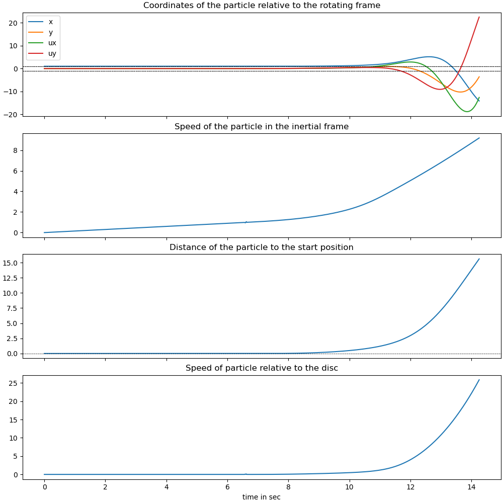
ax[0].set_title('Coordinates of the particle relative to the rotating frame')
ax[1].set_title('Speed of the particle in the inertial frame')
ax[2].set_title('Distance of the particle to the start position')
ax[3].set_xlabel('time in sec')

ax[3].plot(times, rel_speed_np)
_ = ax[3].set_title('Speed of particle relative to the disc')

Animate the System

fps = 15
r_disc = 15

t_arr = times
state_sol = CubicSpline(t_arr, resultat)

Pl, Pr, Pu, Pd = sm.symbols('Pl Pr Pu Pd', cls=me.Point)
Pl.set_pos(O, -r_disc*A.x)
Pr.set_pos(O, r_disc*A.x)
Pu.set_pos(O, r_disc*A.y)
Pd.set_pos(O, -r_disc*A.y)


coordinates = P.pos_from(O).to_matrix(N)
for point in (Pl, Pr, Pu, Pd):
    coordinates = coordinates.row_join(point.pos_from(O).to_matrix(N))

coords_lam = sm.lambdify(qL + pL, coordinates, cse=True)


def init_plot():
    fig, ax = plt.subplots(figsize=(6, 6), layout='constrained')
    ax.set_xlim(-r_disc-1, r_disc+1)
    ax.set_ylim(-r_disc-1, r_disc+1)
    ax.set_aspect('equal')
    ax.set_xlabel('x', fontsize=15)
    ax.set_ylabel('y', fontsize=15)

    # draw the spokes
    line1, = ax.plot([], [], lw=1, marker='o', markersize=0, color='black')
    line2, = ax.plot([], [], lw=1, marker='o', markersize=0, color='black')
    line3 = ax.scatter([], [], color='red', s=100, marker='o')
    line4, = ax.plot([], [], color='blue', lw=0.5)
    return fig, ax, line1, line2, line3, line4


fig, ax, line1, line2, line3, line4 = init_plot()

# draw the disc
phi = np.linspace(0, 2*np.pi, 500)
x_phi = r_disc * np.cos(phi)
y_phi = r_disc * np.sin(phi)
ax.plot(x_phi, y_phi, color='black', lw=2)

old_x, old_y = [], []
for i in range(len(times)):
    pL_vals[-1] = times[i]
    old_x.append(coords_lam(*[resultat[i, j] for j in range(len(qL))],
                            *[pL_vals[j] for j in range(len(pL_vals) - 1)],
                            times[i])[0, 0])
    old_y.append(coords_lam(*[resultat[i, j] for j in range(len(qL))],
                            *[pL_vals[j] for j in range(len(pL_vals) - 1)],
                            times[i])[1, 0])


def update(t):
    message = (
        f'Running time {t:.2f} sec \n'
        f'Angular velocity of the disc {omega1 * t:.2f} rad/sec'
        f' \n The blue line is the path of the particle as seen by an observer'
        ' at rest,'
        )

    ax.set_title(message, fontsize=10)

    coords = coords_lam(*state_sol(t), *[pL_vals[j]
                                         for j in range(len(pL_vals) - 1)], t)
    line1.set_data([coords[0, 1], coords[0, 2]], [coords[1, 1], coords[1, 2]])
    line2.set_data([coords[0, 3], coords[0, 4]], [coords[1, 3], coords[1, 4]])
    line3.set_offsets([coords[0, 0], coords[1, 0]])
    idx = np.argmax(times >= t)
    points_x = old_x[:idx]
    points_y = old_y[:idx]
    line4.set_data(points_x, points_y)


animation = FuncAnimation(fig, update,
                          frames=np.arange(0.0, t_arr[-1], 1/fps),
                          interval=1000/fps, blit=False)

plt.show()

Once Loop Reflect