Note
Go to the end to download the full example code.
Two Connected Balls rolling on Uneven Surface
Objectives
Show how to use Hiller / Anantharaman’s formalism modified for system with both holonomic and nonholonomic constraints.
Show how to use solve_ivp and Sundials IDA for solving differential-algebraic equations.
Description
Two balls with mass \(m_L\) and \(m_R\) and radii \(r_L\) and \(r_R\) are connected by an axle with mass \(m_P\). The balls can rotate freely around the axle. (Maybe the axle is connected by two cups) Particles of mass \(m_P\) are located on the balls. The balls must roll on a smooth surface without slipping.
Notes
The modified Hiller / Anantharam’s formalism was given by Jonas Breuling (private communication).
I used quaternions to represent the orientation of the balls. Regular angles may have lead to gimbal locks, which IDA seemed to be able to handle, but not so solve_dae.
The description of the system may look a bit odd for users used to Kane’s method. This was done so the coordinates of the contact points appear in the formulation.
The axle must have a mass, otherwise \(q_2\) and \(q_3\) will not be in EOMs of the free system.
It is important that the coordinates in \(q_{\text{independent}} + q_{\text{dependent}}\) and in \(u_{\text{independent}} + u_{\text{dependent}}\) appear in the same sequence. (This may be avoided with a transformation matrix, I did not try it.)
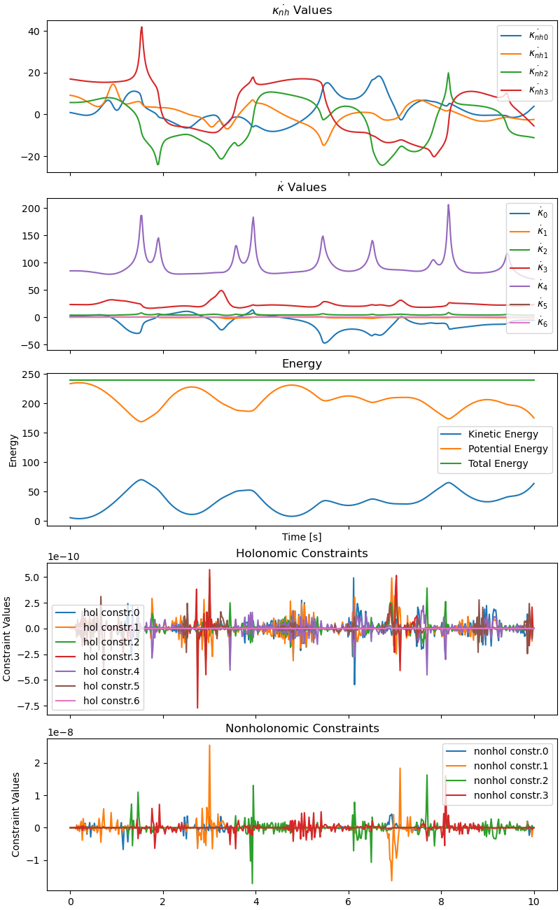
If the constancy of the total energy, absent any friction or driving forces, is a measure of the accuracy of the simulation, it seems that solve_dae, at least with stages = 5 seems more accurate than IDA.
States
\(qL_0, qL_1, qL_2, qL_3\) : Quaternion coordinates representing the orientation of the left ball.
\(qR_0, qR_1, qR_2, qR_3\) : Quaternion coordinates representing the orientation of the right ball.
\(uqL_0, uqL_1, uqL_2, uqL_3\) : Quaternion speeds of the left ball.
\(uqR_0, uqR_1, uqR_2, uqR_3\) : Quaternion speeds of the right ball.
\(q_2, q_3\) : Generalized coordinates of the axle. Note: the axle does not rotate around its own axis.
\(u_2, u_3\) : Generalized speeds of the axle.
\(x_L, y_L, z_L\) : Position coordinates of the contact point on the left ball.
\(x_R, y_R, z_R\) : Position coordinates of the contact point on the right ball.
\(ux_L, uy_L, uz_L\) : Speeds of the contact point on the left ball.
\(ux_R, uy_R, uz_R\) : Speeds of the contact point on the right ball.
Parameters
\(m_L, m_R\) : Masses of the left and right balls.
\(r_L, r_R\) : Radii of the left and right balls.
\(m_P\) : Mass of the particles on the balls.
\(m_{axle}\) : Mass of the axle.
\(l_{axle}\) : Length of the axle.
\(g\) : Gravitational acceleration. In the negative \(z\) direction.
\(amplitude\) : Amplitude of the surface undulations.
\(frequenz\) : Frequency of the surface undulations.
\(friktion\) : Coefficient of rotationalfriction between the balls and the axle.
\(FL_x, FL_y, FL_z\) : Components of the force on the left ball.
\(FR_x, FR_y, FR_z\) : Components of the force on the right ball.
import sympy as sm
import sympy.physics.mechanics as me
import numpy as np
import matplotlib.pyplot as plt
from scipy.interpolate import interp1d
from scipy.optimize import root
from solve_dae.integrate import solve_dae, consistent_initial_conditions
from matplotlib.animation import FuncAnimation
from matplotlib.patches import Circle
from scikits.odes import dae
Define the surface.
x_h, y_h = sm.symbols('x_h y_h')
rumpel = 2
info = False
def gesamt(x, y, amplitude, frequenz, rumpel):
strasse = sum([amplitude/j * (sm.sin(j*frequenz*sm.pi * x) +
sm.sin(j*frequenz*sm.pi * y))
for j in range(1, rumpel)])
return strasse
def gesamt_plot(x_h, y_h, amplitude, frequenz):
return sum([amplitude/j * (sm.sin(j*frequenz*sm.pi * x_h) +
sm.sin(j*frequenz*sm.pi * y_h))
for j in range(1, rumpel)])
Unconstrained System
Nf, AXf, ALf, ARf = sm.symbols('Nf AXf ALf ARf', cls=me.ReferenceFrame)
Of, DmcLf, DmcRf, CPLf, CPRf, PLf, PRf, P_axf = sm.symbols(
'Of DmcLf DmcRf CPLf CPRf PLf PRf P_axf', cls=me.Point)
t = me.dynamicsymbols._t
Of.set_vel(Nf, 0)
Rotational coordinates of left an right balls and the angular velocities.
qL0, qL1, qL2, qL3, qR0, qR1, qR2, qR3 = me.dynamicsymbols(
'qL0 qL1 qL2 qL3 qR0, qR1 qR2 qR3')
uL0, uL1, uL2, uL3, uR0, uR1, uR2, uR3 = me.dynamicsymbols(
'uL0 uL1 uL2 uL3 uR0 uR1 uR2 uR3')
Generalized coordinates and their corresponding speeds of the axle.
q2, q3, u2, u3 = me.dynamicsymbols('q2 q3 u2 u3')
Position and speed of CPL, CPR.
xL, yL, zL, uxL, uyL, uzL = me.dynamicsymbols('xL yL zL uxL uyL uzL')
xR, yR, zR, uxR, uyR, uzR = me.dynamicsymbols('xR yR zR uxR uyR uzR')
Parameters of the system.
rL, rR, mL, mR, mP, g, lax, friktion = sm.symbols(
'rL rR mL mR mP g lax friktion')
amplitude, frequenz = sm.symbols('amplitude frequenz')
Define the axle, it does not rotate around itself.
AXf.orient_body_fixed(Nf, [q3, q2, 0], 'ZYX')
Body fixed frame of left ball.
ALf.orient_quaternion(AXf, [qL0, qL1, qL2, qL3])
Body fixed frame of right ball.
ARf.orient_quaternion(AXf, [qR0, qR1, qR2, qR3])
Left and right contact points.
CPLf.set_pos(Of, xL * Nf.x + yL * Nf.y + zL * Nf.z)
CPRf.set_pos(Of, xR * Nf.x + yR * Nf.y + zR * Nf.z)
Vectors pointing from the contact points to the centers of the balls.
nLf = (-gesamt(xL, yL, amplitude, frequenz, rumpel).diff(xL) * Nf.x -
gesamt(xL, yL, amplitude, frequenz, rumpel).diff(yL) * Nf.y +
Nf.z).normalize()
nRf = (-gesamt(xR, yR, amplitude, frequenz, rumpel).diff(xR) * Nf.x -
gesamt(xR, yR, amplitude, frequenz, rumpel).diff(yR) * Nf.y +
Nf.z).normalize()
Define the location of the centers of the balls.
DmcLf.set_pos(CPLf, rL * nLf)
DmcRf.set_pos(CPRf, rR * nRf)
Place the particles and the center of the axle.
PLf.set_pos(DmcLf, rL * ALf.y)
PLf.v2pt_theory(DmcLf, Nf, ALf)
PRf.set_pos(DmcRf, rR * ARf.y)
PRf.v2pt_theory(DmcRf, Nf, ARf)
P_axf.set_pos(DmcLf, lax/2 * AXf.x)
_ = P_axf.v2pt_theory(DmcLf, Nf, AXf)
Form the bodies.
Balls.
iXXL = 2 / 5 * mL * rL**2
iYYL = iXXL
iZZL = iXXL
iXXR = 2 / 5 * mR * rR**2
iYYR = iXXR
iZZR = iXXR
Axle.
iXX_ax = 0
iYY_ax = 1/12 * mP * lax**2
iZZ_ax = iYY_ax
inertiaL = me.inertia(ALf, iXXL, iYYL, iZZL)
inertiaR = me.inertia(ARf, iXXR, iYYR, iZZR)
inertia_ax = me.inertia(AXf, iXX_ax, iYY_ax, iZZ_ax)
ballLf = me.RigidBody('ballLf', DmcLf, ALf, mL, (inertiaL, DmcLf))
ballRf = me.RigidBody('ballRf', DmcRf, ARf, mR, (inertiaR, DmcRf))
pLaf = me.Particle('pLaf', PLf, mP)
pRaf = me.Particle('pRaf', PRf, mP)
axlef = me.RigidBody('axlef', P_axf, AXf, mP, (inertia_ax, P_axf))
bodiesf = [ballLf, ballRf, pLaf, pRaf, axlef]
Applied external forces.
FLx, FLy, FRx, FRy = sm.symbols('FLx FLy FRx FRy')
Force list.
FLf = [
(DmcLf, -mL * g * Nf.z + FLx * Nf.x + FLy * Nf.y),
(DmcRf, -mR * g * Nf.z + FRx * Nf.x + FRy * Nf.y),
(PLf, -mP * g * Nf.z),
(PRf, -mP * g * Nf.z),
(P_axf, -mP * g * Nf.z),
(ALf, -friktion * ALf.ang_vel_in(Nf)),
(ARf, -friktion * ARf.ang_vel_in(Nf)),
]
Independent and dependent coordinates and speeds of the constrained system.
q_indf = [qL1, qL2, qL3, qR3, q3, qR1, qR2, xL, yL]
q_depf = [zL, xR, yR, zR, q2, qL0, qR0]
u_indf = [uL1, uL2, uL3, uR3, u3]
u_depf = [uR1, uR2, uxL, uyL, uzL, uxR, uyR, uzR, u2, uL0, uR0]
Combine independent and dependent coordinates and speeds for the free system.
q_ind_free = ([qL1, qL2, qL3, qR3, q3, qR1, qR2, xL, yL] +
[zL, xR, yR, zR, q2, qL0, qR0])
u_ind_free = ([uL1, uL2, uL3, uR3, u3] +
[uR1, uR2, uxL, uyL, uzL, uxR, uyR, uzR, u2, uL0, uR0])
Kane’s method.
kd_free = sm.Matrix([i.diff(t) - j
for i, j in zip(q_ind_free, u_ind_free)])
kane_free = me.KanesMethod(
Nf,
q_ind_free,
u_ind_free,
kd_eqs=kd_free,
)
fr_free, frstar_free = kane_free.kanes_equations(bodiesf, FLf)
MM_free = kane_free.mass_matrix_full
force_free = kane_free.forcing_full
RHS = kane_free.rhs()
if info:
print(f"mass matrix has {sm.count_ops(MM_free):,} operations, "
f"{sm.count_ops(sm.cse(MM_free)[0]):,} operations after cse")
print(f"force vector has {sm.count_ops(force_free):,} operations, "
f"{sm.count_ops(sm.cse(force_free)[0]):,} operations after cse")
print(me.find_dynamicsymbols(MM_free))
print(me.find_dynamicsymbols(force_free), '\n')
kin_dict_free = {i.diff(t): j for i, j in zip(q_ind_free, u_ind_free)}
Set parameters and initial conditions.
Parameters.
rL1 = 1.0
rR1 = 2.0
mL1 = 1.0
mR1 = (rR1 / rL1)**3 * mL1
mP1 = 1.0
g1 = 9.81
lax1 = 5.0
friktion1 = 0.0
amplitude1 = 0.35
frequenz1 = 0.35
FLx1 = 0.0
FLy1 = 0.0
FRx1 = 0.0
FRy1 = 0.0
pL_vals = [rL1, rR1, mL1, mR1, mP1, g1, lax1, friktion1, amplitude1,
frequenz1, FLx1, FLy1, FRx1, FRy1]
Set independent coordinates
q_indf = [qL1, qL2, qL3, qR3, q3, qR1, qR2, xL, yL]
qL11 = 0.0
qL21 = 0.0
qL31 = 0.0
qR11 = 0.0
qR21 = 0.0
qR31 = 0.0
q31 = np.deg2rad(0)
xL1 = 0.0
yL1 = 0.0
q1_ind = [qL11, qL21, qL31, qR31, q31, qR11, qR21, xL1, yL1]
Provisionally set the dependent coordinates.
q_depf = [zL, xR, yR, zR, q2, qL0, qR0]
q1_dep = [1.0] * 7
Set independent speeds.
u_indf = [uL1, uL2, uL3, uR3, u3]
uL11 = 0.5
uL21 = 0.0
uL31 = 0.0
uR31 = 0.0
u31 = 0.0
u1_ind = [uL11, uL21, uL31, uR31, u31]
Provisionally set the dependent speeds.
u_depf = [uR1, uR2, uxL, uyL, uzL, uxR, uyR, uzR, u2, uL0, uR0]
u1_dep = [0] * 11
Set up the Constraints
Distance between DmcL and DmcR must be lax along the AX.x direction.
distanz = DmcRf.pos_from(DmcLf)
hol1f = distanz.dot(AXf.x) - lax
hol2f = distanz.dot(AXf.y)
hol3f = distanz.dot(AXf.z)
Contact points must be on the surface.
hol4f = (CPLf.pos_from(Of).dot(Nf.z) -
gesamt(xL, yL, amplitude, frequenz, rumpel))
hol5f = (CPRf.pos_from(Of).dot(Nf.z) -
gesamt(xR, yR, amplitude, frequenz, rumpel))
Quaternion constraints.
hol6f = qL0**2 + qL1**2 + qL2**2 + qL3**2 - 1
hol7f = qR0**2 + qR1**2 + qR2**2 + qR3**2 - 1
hol_constrf = sm.Matrix([hol1f, hol2f, hol3f, hol4f, hol5f, hol6f, hol7f])
No slip conditions.
CPLf.set_vel(Nf, DmcLf.vel(Nf) + ALf.ang_vel_in(Nf).cross(-rL*nLf))
CPRf.set_vel(Nf, DmcRf.vel(Nf) + ARf.ang_vel_in(Nf).cross(-rR*nRf))
vel_CPLf = CPLf.vel(Nf)
vel_CPRf = CPRf.vel(Nf)
nonhol_constrf = sm.Matrix([
vel_CPLf.dot(Nf.x),
vel_CPLf.dot(Nf.y),
vel_CPRf.dot(Nf.x),
vel_CPRf.dot(Nf.y),
])
Compile some functions.
qLLf = q_ind_free + u_ind_free
pLLf = [rL, rR, mL, mR, mP, g, lax, friktion, amplitude, frequenz,
FLx, FLy, FRx, FRy]
Needed to get the dependent gen. coordinates
hol_constr_lamf = sm.lambdify(q_depf + q_indf + pLLf, hol_constrf, cse=True)
Needed to get the dependent velocities.
velocity_constrf = hol_constrf.diff(t).col_join(nonhol_constrf)
velocity_constrf = me.msubs(velocity_constrf, kin_dict_free)
A_udepf, b_udepf = sm.linear_eq_to_matrix(velocity_constrf, u_depf)
A_udep_lamf = sm.lambdify(q_depf + q_indf + u_indf + pLLf, A_udepf, cse=True)
b_udep_lamf = sm.lambdify(q_depf + q_indf + u_indf + pLLf, b_udepf, cse=True)
For checking how well the constraints are kept.
hol_plot_lamf = sm.lambdify(qLLf + pLLf, hol_constrf, cse=True)
nonhol_constrf = me.msubs(nonhol_constrf, kin_dict_free)
nonhol_plot_lamf = sm.lambdify(qLLf + pLLf, nonhol_constrf, cse=True)
Check the energies, total energy should be zero in friktion = 0.
kin_energyf = sum([body.kinetic_energy(Nf).subs(kin_dict_free)
for body in bodiesf])
pot_energyf = sum([g * body.mass * body.masscenter.pos_from(Of).dot(Nf.z)
for body in bodiesf])
kin_lamf = sm.lambdify(qLLf + pLLf, kin_energyf, cse=True)
pot_lamf = sm.lambdify(qLLf + pLLf, pot_energyf, cse=True)
Set up Hiller / Anatharaman’s modified formalism.
Holonomic constraint: \(g(q) \equiv 0\). Set \(W = \left( \dfrac{\partial{g(q)}}{\partial{q}} \right)^T = 0\), \(W \in \\R^{16 \times 7}\)
Nonholonomic constraint: \(A(q) \cdot u \equiv 0\), \(A \in \\R^{4 \times 16}\)
\(F_0\) = \(\dot{q} - u - W \cdot \dot{\nu}\) \(\in \\R^{16}\)
\(F_1\) = \(M \dot{u} - h - W \dot{\kappa} - A^T \dot{\kappa_{nh}}\) \(\in \\R^{16}\)
\(F_2\) = \(g(q)\) \(\in \\R^{7}\)
\(F_3\) = \(\dfrac{d}{dt} (q(q)\) \(\in \\R^{7}\)
\(F_4\) = \(A(q) \cdot{u}\) \(\in \\R^{4}\)
Lagrange multipliers.
kappa = [me.dynamicsymbols('kappa_' + str(i)) for i in range(7)]
kappadt = [k.diff(t) for k in kappa]
kappanh = [me.dynamicsymbols('kappanh_nh_' + str(i)) for i in range(4)]
kappanhdt = [k.diff(t) for k in kappanh]
nu = [me.dynamicsymbols('nu' + str(i)) for i in range(7)]
nudt = [g.diff(t) for g in nu]
Set W as above.
W_free = hol_constrf.jacobian(q_ind_free)
W_free = me.msubs(W_free, kin_dict_free)
W_free = W_free.T
First line of the equation: F0
F0 = kd_free - W_free * sm.Matrix(nudt)
Second line of the equation: F1
get A_free
nonhol_constrf = me.msubs(nonhol_constrf, kin_dict_free)
A_free, _ = sm.linear_eq_to_matrix(nonhol_constrf, u_ind_free)
EOMs of the free system.
MM_free = kane_free.mass_matrix
force_free = kane_free.forcing
F1 = (MM_free * sm.Matrix([i.diff(t) for i in u_ind_free]) -
force_free -
W_free * sm.Matrix(kappadt) -
A_free.T * sm.Matrix(kappanhdt))
Third line of the equation: F2
F2 = hol_constrf
Forth line of the equation: F3
F3 = me.msubs(hol_constrf.diff(t), kin_dict_free)
Fifth line of the equation: F4
F4 = me.msubs(nonhol_constrf, kin_dict_free)
Needed for solve_dae and for IDA
v = [me.dynamicsymbols('v' + str(i)) for i in range(16 + 16 + 7 + 7 + 4)]
vp = [me.dynamicsymbols('vp' + str(i)) for i in range(16 + 16 + 7 + 7 + 4)]
v_dict = {i: j for i, j in zip(q_ind_free + u_ind_free +
kappa + kappanh + nu, v)}
vp_dict = {i.diff(t): j for i, j in zip(q_ind_free + u_ind_free +
kappa + kappanh + nu, vp)}
It is important to substitute in sequence as shown.
F0 = me.msubs(F0, v_dict)
F0 = me.msubs(F0, vp_dict)
F1 = me.msubs(F1, v_dict)
F1 = me.msubs(F1, vp_dict)
F2 = me.msubs(F2, v_dict)
F2 = me.msubs(F2, vp_dict)
F3 = me.msubs(F3, v_dict)
F3 = me.msubs(F3, vp_dict)
F4 = me.msubs(F4, v_dict)
F4 = me.msubs(F4, vp_dict)
Compilation.
F0_lam = sm.lambdify(v + vp + pLLf, F0, cse=True)
F1_lam = sm.lambdify(v + vp + pLLf, F1, cse=True)
F2_lam = sm.lambdify(v + vp + pLLf, F2, cse=True)
F3_lam = sm.lambdify(v + vp + pLLf, F3, cse=True)
F4_lam = sm.lambdify(v + vp + pLLf, F4, cse=True)
A_free_lamf = sm.lambdify(qLLf + pLLf, A_free, cse=True)
constr_lamf = sm.lambdify(qLLf + pLLf, hol_constrf, cse=True)
nonhol_constr_lamf = sm.lambdify(qLLf + pLLf, nonhol_constrf, cse=True)
Calculate the dependent coordiantes.
def hol_depf(x0, args):
return hol_constr_lamf(*x0, *args).squeeze()
x0_guess = list(q1_dep) # NOT zeros: d(q0^2-1)/dq0 = 0 at q0 = 0
args = q1_ind + pL_vals
for i in range(2):
res = root(hol_depf, x0_guess, args)
x0_guess = res.x
print(res.message, '\n')
q1_depf = res.x
for i in range(len(q_depf)):
print(f"{q_depf[i]} = {q1_depf[i]:.3e}")
The solution converged.
zL(t) = 0.000e+00
xR(t) = -4.775e+00
yR(t) = 3.282e-01
zR(t) = 4.242e-01
q2(t) = -2.859e+00
qL0(t) = 1.000e+00
qR0(t) = 1.000e+00
Calculate dependent speeds.
print("condition of A_udepf:", np.linalg.cond(A_udep_lamf(*q1_depf, *q1_ind,
*u1_ind, *pL_vals)),
'\n')
res = np.linalg.solve(A_udep_lamf(*q1_depf, *q1_ind, *u1_ind, *pL_vals),
b_udep_lamf(*q1_depf, *q1_ind, *u1_ind, *pL_vals))
u1_depf = []
for i in range(len(u_depf)):
u1_depf.append(res[i][0])
print(f"{u_depf[i]} = {res[i][0]:.3e}")
x0 = q1_ind + list(q1_depf) + u1_ind + list(u1_depf)
condition of A_udepf: 10.048649680036956
uR1(t) = 2.236e-01
uR2(t) = 2.138e-03
uxL(t) = 8.759e-02
uyL(t) = 7.490e-01
uzL(t) = 3.220e-01
uxR(t) = 5.267e-02
uyR(t) = 6.030e-01
uzR(t) = 2.275e-01
u2(t) = -7.736e-03
uL0(t) = 0.000e+00
uR0(t) = 0.000e+00
Integrate with solve_dae
v0 = np.concatenate([x0, np.zeros(len(kappa) + len(kappanh) + len(nu))])
vp0 = np.zeros(len(v0))
Define the system of equations for the DAE solver.
def F(t, v, vp):
return np.concatenate([F0_lam(*v, *vp, *pL_vals).ravel(),
F1_lam(*v, *vp, *pL_vals).ravel(),
F2_lam(*v, *vp, *pL_vals).ravel(),
F3_lam(*v, *vp, *pL_vals).ravel(),
F4_lam(*v, *vp, *pL_vals).ravel()])
Get consistent initial conditions.
v01, vp01, f0 = consistent_initial_conditions(F, 0.0, v0, vp0)
f0 = F(0.0, v01, vp01)
print(f"||F(t0)||: {np.linalg.norm(f0):.3e}")
||F(t0)||: 3.649e-14
Safe them for IDA.
v001, vp001 = v01.copy(), vp01.copy()
Set solver parameters and integrate the DAE.
atol = 1e-9
rtol = 1e-9
tf = 10.0
schritte = 500
t_eval = np.linspace(0, tf, schritte)
\(\kappa\), \(\kappa_{nh}\) and \(\nu\) only enter through their derivatives, their errors are of no concern.
atol_dae = np.full(50, atol)
atol_dae[32:50] = 1.e3
Number of stages for the Radau method. Must be an odd number. Only works Radau, mot with BDF.
stages = 5
Solve the DAE system.
sol = solve_dae(F, [0, tf], v01, vp01, atol=atol_dae, rtol=rtol,
method='Radau',
t_eval=t_eval,
stages=stages,
)
success = sol.success
message = sol.message
print(f"success: {success}")
print(f"message: {message}")
print(f"nfev: {sol.nfev}")
print(f"njev: {sol.njev}")
print(f"nlu: {sol.nlu}")
C:\Users\Peter\anaconda3\envs\pst-notebooks-pydy\Lib\site-packages\scipy\integrate\_ivp\common.py:357: RuntimeWarning: overflow encountered in multiply
h_new = (y[ind] + new_factor * y_scale[ind]) - y[ind]
C:\Users\Peter\anaconda3\envs\pst-notebooks-pydy\Lib\site-packages\scipy\integrate\_ivp\common.py:326: RuntimeWarning: overflow encountered in multiply
h = (y + factor * y_scale) - y
C:\Users\Peter\anaconda3\envs\pst-notebooks-pydy\Lib\site-packages\scipy\integrate\_ivp\common.py:356: RuntimeWarning: overflow encountered in multiply
new_factor = NUM_JAC_FACTOR_INCREASE * factor[ind]
C:\Users\Peter\anaconda3\envs\pst-notebooks-pydy\Lib\site-packages\scipy\integrate\_ivp\common.py:378: RuntimeWarning: overflow encountered in multiply
factor[max_diff < NUM_JAC_DIFF_SMALL * scale] *= NUM_JAC_FACTOR_INCREASE
success: True
message: The solver successfully reached the end of the integration interval.
nfev: 22336
njev: 470
nlu: 1467
Plot some results.
def plot_simulation_results(times, valuesy, valuesyp):
fig, ax = plt.subplots(5, 1, figsize=(8, 13), layout='constrained',
sharex=True)
kin_np = np.array([kin_lamf(*valuesy[0: 32, i], *pL_vals)
for i in range(valuesy.shape[1])])
pot_np = np.array([pot_lamf(*valuesy[0: 32, i], *pL_vals)
for i in range(valuesy.shape[1])])
total_np = kin_np + pot_np
for i in range(39, 43):
ax[0].plot(times, valuesyp[i, :],
label='$\dot{\kappa_{nh}}_{' + str(i-39) + '}$')
ax[0].set_title('$\dot{\kappa_{nh}}$ Values')
ax[0].legend()
for i in range(32, 39):
ax[1].plot(times, valuesyp[i, :],
label='$\dot{\kappa}_{' + str(i-32) + '}$')
ax[1].set_title('$\dot \kappa$ Values')
ax[1].legend()
ax[2].plot(times, kin_np, label='Kinetic Energy')
ax[2].plot(times, pot_np, label='Potential Energy')
ax[2].plot(times, total_np, label='Total Energy')
ax[2].set_xlabel('Time [s]')
ax[2].set_ylabel('Energy')
ax[2].set_title('Energy')
ax[2].legend()
for i in range(7):
ax[3].plot(times, [hol_plot_lamf(*valuesy[0:32, j], *pL_vals)[i]
for j in range(valuesy.shape[1])],
label='hol constr.' + str(i))
ax[3].set_ylabel('Constraint Values')
ax[3].set_title('Holonomic Constraints')
ax[3].legend()
for i in range(4):
ax[4].plot(times, [nonhol_plot_lamf(*valuesy[0:32, j], *pL_vals)[i]
for j in range(valuesy.shape[1])],
label='nonhol constr.' + str(i))
ax[4].set_ylabel('Constraint Values')
ax[4].set_title('Nonholonomic Constraints')
ax[4].legend()
if friktion1 == 0 and FLx1 == 0 and FLy1 == 0 and FRx1 == 0 and FRy1 == 0:
delta_energy = (np.max(total_np) - np.min(total_np)) / np.max(total_np)
print("Deviation of total energy from being constant: "
f"{delta_energy:.3e}")
plot_simulation_results(sol.t, sol.y, sol.yp)
C:\Users\Peter\github_repos\pst-notebooks\gallery\plot_balls_on_axle.py:631: SyntaxWarning: invalid escape sequence '\d'
label='$\dot{\kappa_{nh}}_{' + str(i-39) + '}$')
C:\Users\Peter\github_repos\pst-notebooks\gallery\plot_balls_on_axle.py:632: SyntaxWarning: invalid escape sequence '\d'
ax[0].set_title('$\dot{\kappa_{nh}}$ Values')
C:\Users\Peter\github_repos\pst-notebooks\gallery\plot_balls_on_axle.py:637: SyntaxWarning: invalid escape sequence '\d'
label='$\dot{\kappa}_{' + str(i-32) + '}$')
C:\Users\Peter\github_repos\pst-notebooks\gallery\plot_balls_on_axle.py:638: SyntaxWarning: invalid escape sequence '\d'
ax[1].set_title('$\dot \kappa$ Values')
Deviation of total energy from being constant: 3.606e-09
Integrate with IDA
result = np.empty(50)
def residual(t, v, vp, result):
result[0: 16] = F0_lam(*v, *vp, *pL_vals).squeeze()
result[16: 32] = F1_lam(*v, *vp, *pL_vals).squeeze()
result[32: 39] = F2_lam(*v, *vp, *pL_vals).squeeze()
result[39: 46] = F3_lam(*v, *vp, *pL_vals).squeeze()
result[46: 50] = F4_lam(*v, *vp, *pL_vals).squeeze()
f0 = residual(0.0, v001, vp001, result)
print('norm of residual with the initial values', np.linalg.norm(result))
solver = dae(
"ida",
residual,
old_api=False,
rtol=rtol,
atol=atol_dae,
)
tout = np.linspace(0.0, tf, schritte)
solution_i = solver.solve(tout, v001, vp001)
print(solution_i.message)
t_arr = solution_i.values.t
y_arr = solution_i.values.y
yp_arr = solution_i.values.ydot
norm of residual with the initial values 3.649337892550362e-14
No module named 'scikits_odes_daepack'
No module named 'scikits_odes_daepack'
Successful function return.
Plot some results.
plot_simulation_results(t_arr.T, y_arr.T, yp_arr.T)
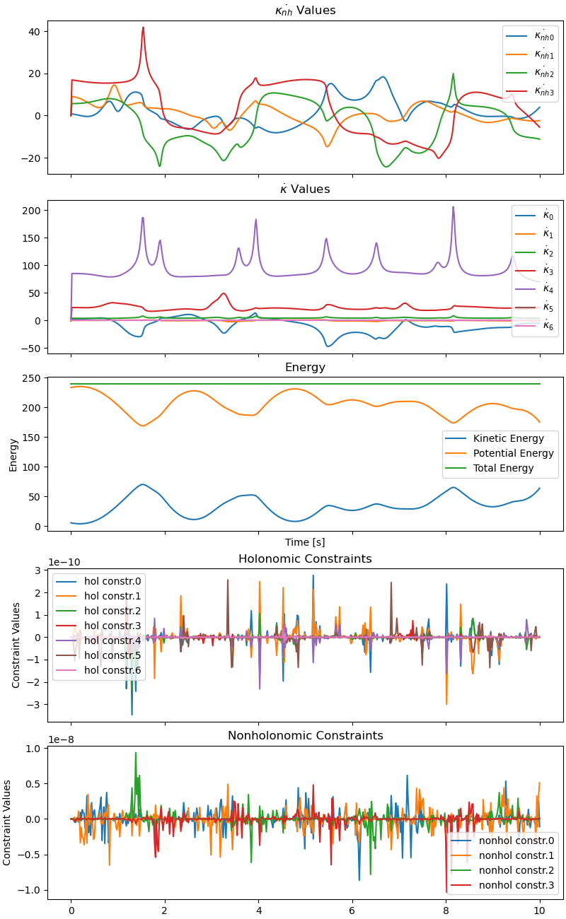
Deviation of total energy from being constant: 8.237e-08
Animation
fps = 10
time_arr = sol.t
state_sol = interp1d(time_arr, sol.y.T, kind='cubic', axis=0)
PLh, PRh = sm.symbols('PLh PRh', cls=me.Point)
PLh.set_pos(DmcLf, rL * AXf.x)
PRh.set_pos(DmcRf, -rR * AXf.x)
coordinates = DmcLf.pos_from(Of).to_matrix(Nf)
for point in (DmcRf, PLf, PRf, PLh, PRh):
coordinates = coordinates.row_join(point.pos_from(Of).to_matrix(Nf))
coords_lam = sm.lambdify(qLLf + pLLf, coordinates, cse=True)
max_x = np.max(sol.y.T[:, 7]) + lax1 + max(rL1, rR1)
max_y = np.max(sol.y.T[:, 8]) + max(rL1, rR1)
min_x = np.min(sol.y.T[:, 7]) - lax1 - max(rL1, rR1)
min_y = np.min(sol.y.T[:, 8]) - max(rL1, rR1)
gesamt_plot_lam = sm.lambdify([x_h, y_h, amplitude, frequenz],
gesamt_plot(x_h, y_h, amplitude, frequenz),
cse=True)
max_radius = 2.0 * max(rL1, rR1)
xx = np.linspace(min_x-max_radius, max_x+max_radius, 100)
yy = np.linspace(min_y-max_radius, max_y+max_radius, 100)
XX, YY = np.meshgrid(xx, yy)
ZZ = gesamt_plot_lam(XX, YY, amplitude1, frequenz1)
fig, ax = plt.subplots(figsize=(7, 7))
ax.set_xlim(min_x-max_radius, max_x+max_radius)
ax.set_ylim(min_y-max_radius, max_y+max_radius)
ax.set_aspect('equal')
ax.set_xlabel('x', fontsize=15)
ax.set_ylabel('y', fontsize=15)
cf = ax.contourf(XX, YY, ZZ, levels=50, cmap='viridis')
fig.colorbar(cf, label='z value [m]', shrink=0.75)
line1, = ax.plot([], [], lw=0.5, marker='o', markersize=0, color='blue',
linestyle='--', alpha=1.0)
line4 = ax.scatter([], [], color='black', s=20)
line5 = ax.scatter([], [], color='black', s=20)
# balls represented as circles in 2D.
coords = coords_lam(*state_sol(0)[0: 32], *pL_vals)
discL = Circle((coords[0, 0], coords[1, 0]), radius=rL1, fill=True, lw=2,
color='red', alpha=0.9, edgecolor=None)
ax.add_patch(discL)
discR = Circle((coords[0, 1], coords[1, 1]), radius=rR1, fill=True, lw=2,
color='yellow', alpha=0.9, edgecolor=None)
ax.add_patch(discR)
def update(t):
message = (f'Running time {t:.2f} sec \n'
f'The left ball is red with radius {rL1}, the '
f'right ball is yellow \n with radius {rR1},'
f' The black dots are the particles attached \n to the balls')
ax.set_title(message, fontsize=11)
coords = coords_lam(*state_sol(t)[0: 32], *pL_vals)
line1.set_data([coords[0, 4], coords[0, 5]], [coords[1, 4],
coords[1, 5]])
if coords[2, 2] < coords[2, 0]:
line4.set_alpha(0.5)
else:
line4.set_alpha(1.0)
line4.set_offsets([coords[0, 2], coords[1, 2]])
if coords[2, 3] < coords[2, 1]:
line5.set_alpha(0.5)
else:
line5.set_alpha(1.0)
line5.set_offsets([coords[0, 3], coords[1, 3]])
# update the positions of the circles
discL.center = (coords[0, 0], coords[1, 0])
discR.center = (coords[0, 1], coords[1, 1])
return line1, line4, line5, discL, discR
# Create the animation
animation = FuncAnimation(fig, update,
frames=np.concatenate(
[np.arange(0, sol.t[-1], 1.0/fps), [sol.t[-1]]]),
interval=1000/fps, blit=False)
plt.show()