Note
Go to the end to download the full example code.
Bouncing Ellipse
Objective
Show how to use Hunt-Crossley’s theory of impact on a somewhat non-trivial example.
Description of the Model
A homogenious ellipse of mass \(m\) and semi axes \(a, b\) is dropped or thrown on an uneven street. A particle of mass \(m_o\) may be attached anywhere within th ellipse.
The street is a curve in the X/Y plane, gravitation points in the negative Y - direction.
The impact is modelled using the Hunt-Crossley method, details below.
Notes
The force related terms, such as spring energy and the H-C hysteresis curves take a long time to calculate. Hence this may be suppressed by setting force_display = False.
The integration with the parameters as given takes about 15 min on a decent PC.
The animation may be made smoother by increasing
schrittzahlbelow, at the animation section of the simulation.
Parameters and Variables
\(N\) : inertial frame
\(A\) : frame fixed to the ellipse
\(P_0\) : point fixed in N
\(Dmc\) : center of the ellipse
\(CP_h, CP_{hs}\) : contact points, explained in more detail below.
\(P_o\) : location of the particle fixed to the ellipse
\(q, u\) : angle of rotation of the ellipse, angular speed
\(m_x, m_y, um_x, um_y\) : coordinates of the center of the ellipse, its speeds
\(x\) : X - coordinate of the impact point \(CP_{hs}\) ,of course the Y - coordinate is \(\textrm{gesamt}(x)\)
\(m, m_o\) : mass of the ellipse, of the particle attached to the ellipse
\(a, b\) : semi axes of the ellipse
\(\textrm{amplitude, frequenz}\) : parameters for the street.
\(i_{ZZ}\) : moment of inertia of the ellipse around the Z axis
\(\alpha, \beta\) : determine the location of the particle w.r.t. \(Dmc\)
\(\textrm{reibung}\) : speed dependent friction between the ellipse and the street.
\(\nu, E_Y\) : Poisson’s ratio and Young’s modulus
\(rhodt_{max}\) : speed at the moment of impact, needed for Hunt-Crossley’s method, described below.
import sympy as sm
import sympy.physics.mechanics as me
import numpy as np
from scipy.optimize import minimize, root
from scipy.integrate import solve_ivp
import itertools as itt
from matplotlib import animation
import matplotlib
from matplotlib import patches
import matplotlib.pyplot as plt
matplotlib.rcParams['animation.embed_limit'] = 2**128
force_display = True
m, mo, g, a, b, iZZ, alpha, beta, reibung = sm.symbols(('m, mo, g, a, b, iZZ, '
'alpha, beta, '
'reibung'))
nue, nus, EYe, EYs, ctau = sm.symbols('nue, nus EYe, EYs, ctau')
amplitude, frequenz = sm.symbols('amplitude, frequenz')
x, rhodtmax = sm.symbols('x, rhodtmax')
mx, my, umx, umy = me.dynamicsymbols('mx, my, umx, umy')
q, u = me.dynamicsymbols('q, u')
t = me.dynamicsymbols._t
N, A = sm.symbols('N, A', cls=me.ReferenceFrame)
P0, Dmc, CPh, CPhs, Po = sm.symbols('P0, Dmc, CPh, CPhs, Po', cls=me.Point)
P0.set_vel(N, 0.)
A.orient_axis(N, q, N.z)
A.set_ang_vel(N, u*N.z)
Model the street.
# It is a parabola, open to the top, with superimposed sinus waves.
# Then the radius of the osculating circle is calculated, the formula is from
# the internet.
rumpel = 5 # the higher the number the more 'uneven the street'
def gesamt1(x, amplitude, frequenz):
strasse = sum([amplitude/j * sm.sin(j*frequenz * x)
for j in range(1, rumpel)])
strassen_form = (frequenz/2. * x)**2
gesamt = strassen_form + strasse
return gesamt
r_max = ((sm.S(1.) + (gesamt1(x, amplitude, frequenz).diff(x))**2)**sm.S(3/2) /
gesamt1(x, amplitude, frequenz).diff(x, 2))
Find the Point where the Ellipse Hits the Street
The idea is as follows:
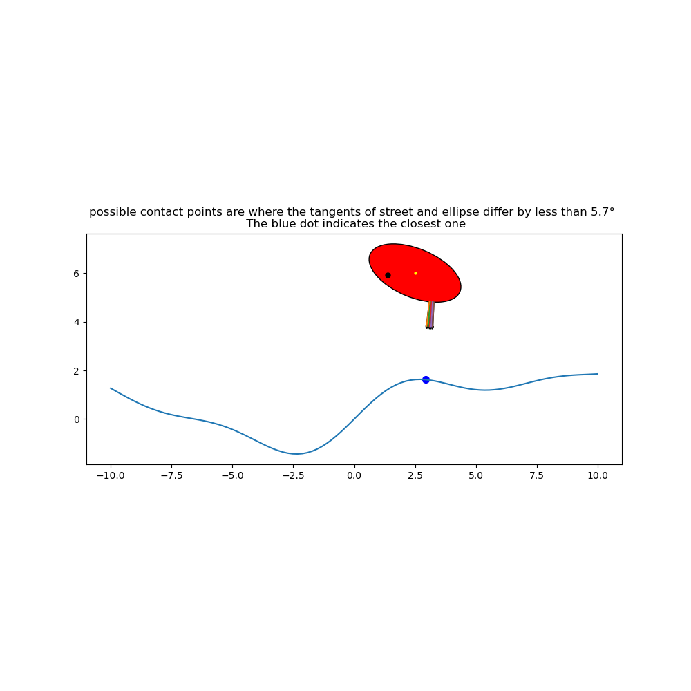
When the ellipse hits the street, the tangent at the ellipse at the hitting point, and the tangent at the street at the hitting point must be parallel. So, look for the point where the ellipse would touch the street if it was ‘inflated’ by just the right amount to touch the street for every point of the integration time. This sequence of potential hitting points will eventually give the real hitting point.
let \(CP_{hs}\) be the point of the street where a multiple of the vector \(\hat n\) which is normal to the tanget of the ellipse at \(CP_h \in \textrm{circumference of ellipse}\) intersects with the street below.
is the tangent of the ellipse at \(CP_h\) parallel to the tangent of the street at \(CP_{hs}\)?
if YES, \(CP_{hs}\) is a potential impact point.
collect all potential impact points, and select the one closest to the ellipse. This is the point the ellipse would touch, if it were ‘blown up’ to just touch the street.
All this has to be done numerically during integration.
In more detail:
To get the derivative of the ellipse at the point \((x, y) \in \textrm{circumference of ellipse}\) calculate: \(\dfrac{d}{dx}(\dfrac{x^2}{a^2} + \dfrac{y^2}{b^2} = 1)\)
to get:
\(\dfrac{dy}{dx} = - \dfrac{b^2}{a^2} \cdot \dfrac{x}{y}\) for \(y \neq 0\)
hence the normalized tanget vector is
\(t_{\textrm{ellipse}} = (\hat{ A.x + \dfrac{dy}{dx} \cdot A.y})\) for \(y \neq 0\)
\(t_{\textrm{ellipse}} = +/- A.y\) for \(y = 0.\)
Therefore the normal vector in the unrotated ellipse is:
\(\hat n = (\hat{ \dfrac{dy}{dx} \cdot A.x - A.y})\) for \(y \neq 0\)
\(\hat n = A.x\) for \(y = 0, x = a\)
\(\hat n = -A.x\) for \(y = 0, x = -a\)
To get \(\hat n\) in the ellipse rotated by q, one calculates: \(\hat n_{\textrm{rotated by q}} = A(q)^T \cdot \hat n\)
Find the location of \(CP_{hs}\) : \(CP_{hs} \in\) gesamt(x, parameters) where the function gesamt(x, parameters) models the street
Let \(l = |{}^{CP_{hd}} r^{CP_h}| = |l \hat n|\), then we get two equations:
\((l\hat n \cdot N.x) = x\)
\((l\hat n \cdot N.y) = gesamt(x),\)
to be solved during each step of the numerical integration. However, during integration solved only if \(\hat n \cdot N.y \leq 0\). For the shape of the street, this seems adequate and reduces running time.
\(\sin(\theta) = | \textrm{tangent}_{\textrm{ellipse}} \times \textrm{tangent}_{\textrm{street}} |\) is taken as a measure how ‘parallel’ the tangents at the collision points are, where the tangents are unit vectors, and \(\theta\) is the angle between them.
Dmc.set_pos(P0, mx*N.x + my*N.y)
Dmc.set_vel(N, umx*N.x + umy*N.y)
# define the 'observer'
Po.set_pos(Dmc, alpha*a*A.x + beta*b*A.y)
Po.v2pt_theory(Dmc, N, A)
# find the vector normal to the tanget at the unrotated ellipse
# at the point CPh
delta, l = sm.symbols('delta, l')
CPhx = a * sm.cos(delta)
CPhy = b * sm.sin(delta)
ausdruckk = (sm.Abs(CPhy) <= 1.e-15)
ausdruckg = (sm.Abs(CPhy) > 1.e-15)
dydx = sm.Piecewise((-b**2/a**2 * CPhx/CPhy, ausdruckg), (1.e15, ausdruckk),
(1., True))
that0 = (A.x + dydx*A.y).normalize()
hilfsx = sm.Piecewise((1., delta == sm.S(0)), (-1., delta == sm.pi),
(-dydx, delta < sm.pi/2.), (-dydx, delta < sm.pi),
(dydx, delta < 3./2.*sm.pi), (dydx, delta < 2.*sm.pi),
(1., True))
hilfsy = sm.Piecewise((0., ausdruckk), (1., delta < sm.pi/2.),
(1., delta < sm.pi), (-1., delta < 3./2.*sm.pi),
(-1, delta < 2.*sm.pi), (1., True))
nhat0 = hilfsx*A.x + hilfsy*A.y
# rotated the normal vector
A1 = A.dcm(N).T
print('A1 = ', '\n', A1, '\n')
nhat1 = A1 @ sm.Matrix([hilfsx, hilfsy, 0.])
that1 = A1 @ sm.Matrix([1., dydx, 0.])
nhat = (nhat1[0]*N.x + nhat1[1]*N.y).normalize()
that = (that1[0]*N.x + that1[1]*N.y).normalize()
print('nhat DS', me.find_dynamicsymbols(nhat, reference_frame=N))
print('nhat FS', nhat.free_symbols(reference_frame=N))
# define CPh and CHhs
CPh.set_pos(Dmc, CPhx*A.x + CPhy*A.y)
CPh.v2pt_theory(Dmc, N, A)
CPhs.set_pos(CPh, l*nhat)
hilfs1 = CPhs.pos_from(P0)
# CPhs_ort to be solved numerically later duering each step of the integration.
CPhs_ort = sm.Matrix([me.dot(hilfs1, N.x) - x, me.dot(hilfs1, N.y)
- gesamt1(x, amplitude, frequenz)])
print('CPhs_ort DS', me.find_dynamicsymbols(CPhs_ort))
print('CPhs_ort FS', CPhs_ort.free_symbols)
print((f'CPhs_ort has {sm.count_ops(CPhs_ort)} operations. After cse it has '
f'{sm.count_ops(sm.cse(CPhs_ort))}'))
strasse = gesamt1(x, amplitude, frequenz)
strassedx = strasse.diff(x)
tangente_strasse = (N.x + strassedx * N.y).normalize()
parallel = (that.cross(tangente_strasse)).magnitude()
print('parallel FS', parallel.free_symbols)
parallel_lam = sm.lambdify([q, mx, my] + [x, delta, a, b, amplitude, frequenz],
parallel, cse=True)
CPhs_ort_lam = sm.lambdify([x, l] + [q, mx, my] + [a, b, amplitude, frequenz,
delta], CPhs_ort, cse=True)
# This is needed only for the plot with the initial conditions
CPha = me.Point('CPha')
CPhe = me.Point('CPhe')
CPha.set_pos(Dmc, CPhx*A.x + CPhy*A.y)
CPhe.set_pos(CPha, 1.*nhat)
liste = [[me.dot(punkt.pos_from(P0), uv) for uv in (N.x, N.y)]
for punkt in (CPha, CPhe)]
liste_lam = sm.lambdify([q, mx, my, delta, a, b], liste, cse=True)
nhat_lam = sm.lambdify([q, delta, a, b],
[me.dot(nhat, N.x), me.dot(nhat, N.y)], cse=True)
senkrecht = me.dot(nhat, that)
senkrecht_lam = sm.lambdify((q, delta, a, b), senkrecht, cse=True)
A1 =
Matrix([[cos(q(t)), -sin(q(t)), 0], [sin(q(t)), cos(q(t)), 0], [0, 0, 1]])
nhat DS {q(t)}
nhat FS {b, t, a, delta}
CPhs_ort DS {mx(t), q(t), my(t)}
CPhs_ort FS {x, b, l, t, a, amplitude, delta, frequenz}
CPhs_ort has 328 operations. After cse it has 81
parallel FS {x, a, b, amplitude, delta, t, frequenz}
Force and Friction on \(CP_h\) during impact
Force acting on \(CP_h\) during impact Hunt_Crossley’s method is used to calculate it.
Hunt Crossley’s method
This article is the reference for the Hunt-Crossley method: https://www.sciencedirect.com/science/article/pii/S0094114X23000782
This is with dissipation during the collision, the general force is given in equation (63) of this article as \(f_n = k_0 \cdot \rho + \chi \cdot \dot \rho\), with \(k_0\) as below, \(\rho\) the penetration, and \(\dot\rho\) the speed of the penetration. In the article it is stated, that \(n = \frac{3}{2}\) is a good choice, it is derived in Hertz’ approach. Of course, \(\rho, \dot\rho\) must be the signed magnitudes of the respective vectors.
A more realistic force is given in (64) as: \(f_n = k_0 \cdot \rho^n + \chi \cdot \rho^n\cdot \dot \rho\), as this avoids discontinuity at the moment of impact.
Hunt and Crossley give this value for \(\chi\), see table 1:
\(\chi = \dfrac{3}{2} \cdot(1 - c_\tau) \cdot \dfrac{k_0}{\dot \rho^{(-)}}\),
where \(c_\tau = \dfrac{v_1^{(+)} - v_2^{(+)}}{v_1^{(-)} - v_2^{(-)}}\),
where \(v_i^{(-)}, v_i^{(+)}\) are the speeds of \(body_i\), before and after the collosion, see (45),
\(\dot\rho^{(-)}\) is the speed right at the time the impact starts.
\(c_\tau\) is an experimental factor, apparently around 0.8 for steel.
Using (64), this results in their expression for the force:
\(f_n = k_0 \cdot \rho^n \left[1 + \dfrac{3}{2} \cdot(1 - c_\tau) \cdot \dfrac{\dot\rho}{\dot\rho^{(-)}}\right]\)
with \(k_0 = \frac{4}{3\cdot(\sigma_1 + \sigma_2)} \cdot \sqrt{\frac{R_1 \cdot R_2}{R_1 + R_2}}\), where
\(\sigma_i = \frac{1 - \nu_i^2}{E_i}\),
with
\(\nu_i\) = Poisson’s ratio, \(E_i\) = Youngs modulus, \(R_1, R_2\) the radii of the colliding bodies, \(\rho\) the penetration depth.
All is near equations (54) and (61) of this article.
Penetration depth \(\rho\):
From the description above, it is clear that \(\rho = |l| \cdot H(-l)\), with \(l\) from above (found numerically) , and \(H(...)\) being the Heaviside function (step function).
Determine \(R_1, R_2\) in the above formulas:
For a function \(y = f(x)\) the signed curvature is: \(\kappa = \dfrac{\frac{d^2}{dx^2} f(x)}{(1 + (\frac{d}{dx} f(x))^2)^ {\frac{3}{2}}}\)
For an ellipse, \(\kappa = \dfrac{a \cdot b}{ \left( \sqrt{a^2 \sin^2(\delta) + b^2 \cos^2(\delta)} \right)^3} > 0 \forall \delta \in [0, 2 \pi)\) where \(\delta\) is the angle from \(A.x\) to the point. As an approximation for \(R_1, R_2\) I take the radius of the osculating circle, which is: \(R_i = \dfrac{1}{\kappa_i}\) If the penetration depth is no too large, this should be o.k. Note,that negative \(R_2\) are allowed: This means, the street is concave from the ellipse’s point of view. At a contact point, either \(R_2 > 0\) or \(|R_2| \leq R_1\) there should be no problems.
Unclear whether this approach is within the validity of the H-C method
Penetration speed
\(\frac{d}{dt} \rho(t)\) Only the component of \(\frac{d}{dt} CP_h(t)\) is relevant, hence: \(\frac{d}{dt} \rho(t) = \frac{d}{dt} CP_h \cdot \hat n\)
spring energy = \(k_0 \cdot \int_{0}^{\rho} k^{3/2}\,dk = k_0 \cdot\frac{2}{5} \cdot \rho^{5/2}\) The article does not give a closed form for the dissipated energy.
Note
\(c_\tau = 1.\) gives Hertz’s solution to the impact problem, also described in the article.
Friction when the ellipse hits the street
It acts on \(CP_h\)
\(|\textrm{friction force}| = |\textrm{impact force}| \cdot \textrm{reibung} \cdot |\bar v(CP_h)\bot \hat n |\) and opposite in direction to the component of \(\bar v(CP_h) \bot \hat n\)
# impact force on :math:`CP_h`
#
# curvature of the ellipse at the point :math:`P((a \cos(\delta) | b
# \sin(\delta))`, from the internet:
kappa1 = (a * b) / (sm.sqrt((a*sm.sin(delta))**2 + (b*sm.cos(delta))**2))**3
# formula for the curvature of a function. From the internet.
hilfs = gesamt1(x, amplitude, frequenz)
hilfsdx = hilfs.diff(x)
hilfsdxdx = hilfsdx.diff(x)
kappa2 = sm.Piecewise((hilfsdxdx**2 / (1. + hilfsdx**2)**1.5, hilfsdxdx != 0.),
(1.e-5, True))
R1 = 1. / kappa1
R2 = 1. / kappa2
sigmae = (1. - nue**2) / EYe
sigmas = (1. - nus**2) / EYs
k0 = 4./3. * 1./(sigmae + sigmas) * sm.sqrt(R1*R2 / (R1 + R2))
rhodt = me.dot(CPh.pos_from(P0).diff(t, N), nhat).subs({
sm.Derivative(mx, t): umx, sm.Derivative(my, t): umy,
sm.Derivative(q, t): u})
rho = sm.Abs(l) * sm.Heaviside(-l, sm.S(0))
print('rhodt DS', me.find_dynamicsymbols(rhodt))
print('rhodt FS', rhodt.free_symbols)
fHC_betrag = (k0 * rho**(3/2) * (1. + 3./2. * (1. - ctau)
* (rhodt) / sm.Abs(rhodtmax)))
# the force is acting on CPh, hence the minus sign.
fHC = fHC_betrag * (-nhat) * sm.Heaviside(-l, sm.S(0))
print('fHC DS', me.find_dynamicsymbols(fHC, reference_frame=N))
print('fHC FS', fHC.free_symbols(reference_frame=N))
# friction force on CPh
that = me.dot(nhat, N.y)*N.x - me.dot(nhat, N.x)*N.y
vCPh = (me.dot(CPh.pos_from(P0).diff(t, N), that)).subs(
{sm.Derivative(mx, t): umx, sm.Derivative(my, t): umy,
sm.Derivative(q, t): u})
F_friction = (fHC.magnitude() * reibung * vCPh * (-that)
* sm.Heaviside(-l, sm.S(0)))
print('F_friction DS', me.find_dynamicsymbols(F_friction, reference_frame=N))
print('F_friction FS', F_friction.free_symbols(reference_frame=N))
rhodt DS {umy(t), q(t), umx(t), u(t)}
rhodt FS {b, t, a, delta}
fHC DS {umx(t), q(t), u(t), umy(t)}
fHC FS {nus, x, l, t, delta, rhodtmax, a, amplitude, EYs, b, EYe, nue, ctau, frequenz}
F_friction DS {umx(t), q(t), u(t), umy(t)}
F_friction FS {nus, x, reibung, ctau, l, t, rhodtmax, a, amplitude, EYs, b, EYe, nue, delta, frequenz}
Kane’s equations.
Ie = me.inertia(A, 0., 0., iZZ)
bodye = me.RigidBody('bodye', Dmc, A, m, (Ie, Dmc))
Poa = me.Particle('Poa', Po, mo)
BODY = [bodye, Poa]
FL = [(Dmc, -m*g*N.y), (Po, -mo*g*N.y), (CPh, fHC), (CPh, F_friction)]
kd = [u - q.diff(t), umx - mx.diff(t), umy - my.diff(t)]
q_ind = [q, mx, my]
u_ind = [u, umx, umy]
KM = me.KanesMethod(N, q_ind=q_ind, u_ind=u_ind, kd_eqs=kd)
(fr, frstar) = KM.kanes_equations(BODY, FL)
MM = KM.mass_matrix_full
force = KM.forcing_full
print('force DS', me.find_dynamicsymbols(force))
print('force free symbols', force.free_symbols)
print((f'force has {sm.count_ops(force)} operations, '
f'{sm.count_ops(sm.cse(force))} operations after cse', '\n'))
print('MM DS', me.find_dynamicsymbols(MM))
print('MM free symbols', MM.free_symbols)
print((f'MM has {sm.count_ops(MM)} operations, {sm.count_ops(sm.cse(MM))} '
f'operations after cse', '\n'))
force DS {q(t), umx(t), u(t), umy(t)}
force free symbols {nus, g, reibung, l, beta, amplitude, b, mo, EYe, nue, alpha, frequenz, x, ctau, t, rhodtmax, a, EYs, m, delta}
('force has 14047 operations, 234 operations after cse', '\n')
MM DS {q(t)}
MM free symbols {m, b, mo, iZZ, t, beta, a, alpha}
('MM has 53 operations, 24 operations after cse', '\n')
Lambdify the functions
Calculate the expressions for the energies.
pot_energie = (m * g * me.dot(Dmc.pos_from(P0), N.y) + mo * g
* me.dot(Po.pos_from(P0), N.y))
kin_energie = sum([koerper.kinetic_energy(N) for koerper in BODY])
spring_energie = 2./5. * k0 * sm.Abs(l)**(5/2) * sm.Heaviside(-l, 0.)
qL = q_ind + u_ind
pL = [x, l, delta] + [m, mo, g, a, b, iZZ, alpha, beta, amplitude,
frequenz, reibung] + [ctau, EYe, EYs, nue, nus, rhodtmax]
MM_lam = sm.lambdify(qL + pL, MM, cse=True)
force_lam = sm.lambdify(qL + pL, force, cse=True)
rhodt_lam = sm.lambdify([q, u, umx, umy] + [a, b, delta], rhodt, cse=True)
gesamt = gesamt1(x, amplitude, frequenz)
gesamt_lam = sm.lambdify([x, amplitude, frequenz], gesamt, cse=True)
Po_ort_lam = sm.lambdify([q, mx, my] + [a, b, alpha, beta],
[me.dot(Po.pos_from(P0), uv)
for uv in (N.x, N.y)], cse=True)
pot_lam = sm.lambdify(qL + pL, pot_energie, cse=True)
kin_lam = sm.lambdify(qL + pL, kin_energie, cse=True)
spring_lam = sm.lambdify(qL + pL, spring_energie, cse=True)
r_max_lam = sm.lambdify([x, amplitude, frequenz], r_max, cse=True)
k0_lam = sm.lambdify(qL + pL, k0*sm.Heaviside(-l, 0), cse=True)
Numerical integration
the parameters and the initial values of independent coordinates are set.
an exception is raised if \(\alpha\) or \(\beta\) are selected such that the particle will be outside of the ellipse.
Check whether the minimum osculating cycle of the street is smaller than max(a, b).
Plot the initial location of the ellipse. This plot also give possible contact points. The closest one is marked on the street. Making \(EY_e\) or \(EY_s\) too large results in a stiff system. The simulation becomes inaccurate, unless max_step is made very small.
# Input parameters
m1 = 1.
mo1 = 1.
g1 = 9.8
a1 = 2.
b1 = 1.
amplitude1 = 1.
frequenz1 = 0.25
reibung1 = 0.1
EYe1 = 1.e4
EYs1 = 1.e7
ctau1 = 0.9
nue1 = 0.28
nus1 = 0.28
alpha1 = 0.5
beta1 = 0.5
q1 = np.pi/8. * 7.
u1 = 5.5
mx1 = 2.5
my1 = 6.
umx1 = 0.
umy1 = -4.75
intervall = 5.0
# max sin(angle) how the tangents of the street and the ellipse may differ
# for a contact point
min_winkel = 0.1
if alpha1**2/a1**2 + beta1**2/b1**2 >= 1.:
raise Exception('Particle is outside the ellipse')
iZZ1 = 0.25 * m1 * (a1**2 + b1**2) # from the internet
# schritte should be close to nfev, the number of times solve_ivp calls
# the function.
schritte = int(intervall * 568.)
# Find the largest admissible r_max, given strasse, amplitude, frequenz
r_max = max(a1**2/b1, b1**2/a1) # max osculating circle of an ellipse
def func2(x, args):
# just needed to get the arguments matching for minimize
return np.abs(r_max_lam(x, *args))
x0 = 0.1 # initial guess
minimal = minimize(func2, x0, [amplitude1, frequenz1])
if r_max < (x111 := minimal.get('fun')):
print(('selected r_max of the ellipse = {} is less than the minimal '
'osculating circle of the street = {:.2f}')
.format(r_max, x111), '\n')
else:
print(('selected r_max of the ellipse = {} is larger than the minimal '
'osculating circle of the street = {:.2f}')
.format(r_max, x111), '\n')
# numerically find x1 = X coordinate of CPhs and l1 := distance
# from CPh to CPhs for the initial condition
# and make a plot of the initial situation
def func_x1_l1(x0, args):
return CPhs_ort_lam(*x0, *args).reshape(2)
delta1 = 0. # of no consequence, any value will do
rhodtmax1 = 1. # dto.
TEST = []
TEST1 = []
x0 = list((-100., 100.))
for epsilon in np.linspace(1.e-15, 2.*np.pi, int(25/min_winkel)):
if nhat_lam(q1, epsilon, a1, b1)[1] <= 0.:
args1 = list((q1, mx1, my1, a1, b1, amplitude1, frequenz1, epsilon))
ergebnis = root(func_x1_l1, x0, args1, method='broyden1')
x0 = ergebnis.x
x1 = x0[0]
if parallel_lam(q1, mx1, my1, x1, epsilon, a1, b1, amplitude1,
frequenz1) < min_winkel:
TEST1.append(liste_lam(q1, mx1, my1, epsilon, a1, b1))
TEST.append((*x0, epsilon))
kontakt = min(TEST, key=lambda k: k[1])
Cax = np.array([TEST1[i][0][0] for i in range(len(TEST1))])
Cay = np.array([TEST1[i][0][1] for i in range(len(TEST1))])
Cex = np.array([TEST1[i][1][0] for i in range(len(TEST1))])
Cey = np.array([TEST1[i][1][1] for i in range(len(TEST1))])
fig, ax = plt.subplots(figsize=(10, 10))
ax.set_aspect('equal')
elli = patches.Ellipse((mx1, my1), width=2.*a1, height=2.*b1,
angle=np.rad2deg(q1), zorder=1, fill=True, color='red',
ec='black')
ax.add_patch(elli)
weite = 10.
ax.plot(mx1, my1, color='yellow', marker='o', markersize=2)
ax.plot(Po_ort_lam(q1, mx1, my1, a1, b1, alpha1, beta1)[0],
Po_ort_lam(q1, mx1, my1, a1, b1, alpha1, beta1)[1], color='black',
marker='o', markersize=5)
ax.plot(kontakt[0], gesamt1(kontakt[0], amplitude1, frequenz1), color='blue',
marker='o', markersize=7)
ax.plot(np.linspace(-weite, weite, 100),
gesamt_lam(np.linspace(-weite, weite, 100), amplitude1, frequenz1))
for i in range(len(Cax)):
x_werte = [Cax[i], Cex[i]]
y_werte = [Cay[i], Cey[i]]
ax.plot(x_werte, y_werte)
ax.arrow(Cax[i], Cay[i], Cex[i]-Cax[i], Cey[i] - Cay[i], shape='full',
width=0.025)
ax.set_title((f'possible contact points are where the tangents of street and '
f'ellipse differ by less than '
f'{np.rad2deg(np.arcsin(min_winkel)):.1f}° \n The blue dot '
f'indicates the closest one'))
pL = [x, l, delta] + [m, mo, g, a, b, iZZ, alpha, beta, amplitude,
frequenz, reibung] + [ctau, EYe, EYs, nue, nus, rhodtmax]
pL_vals = [kontakt[0], kontakt[1], delta1] + \
[m1, mo1, g1, a1, b1, iZZ1, alpha1, beta1, amplitude1,
frequenz1, reibung1] + [ctau1, EYe1, EYs1, nue1, nus1, rhodtmax1]
print('Initial parameters are:', pL_vals, '\n')
y0 = [q1, mx1, my1] + [u1, umx1, umy1]
print('starting values are: ', y0)
selected r_max of the ellipse = 4.0 is larger than the minimal osculating circle of the street = 2.14
Initial parameters are: [np.float64(2.926839986416512), np.float64(3.195954021306725), 0.0, 1.0, 1.0, 9.8, 2.0, 1.0, 1.25, 0.5, 0.5, 1.0, 0.25, 0.1, 0.9, 10000.0, 10000000.0, 0.28, 0.28, 1.0]
starting values are: [2.748893571891069, 2.5, 6.0, 5.5, 0.0, -4.75]
Here the actual integration starts. cut_off determines, after how many failures to find contact points the integration should stop with an exception. This to avoid endless looping of the integration if root does not find a solution.
scipy.optimize.root, but only with method=broyden1 works much better than fsolve. In the preliminary tests, it always found a solution immediately, or else it terminates with an error like ‘jacobian is singular’ or similar.
cut_off = 25
x0 = list((pL_vals[0], pL_vals[1])) # initial guess for fsolve
# root checks zaehler/min_winkel locations around the circumference of the
# ellipse for possible contact points. If this is too crude,
# this number will be tripled, and tried again.
zaehler = 25
zaehler1 = zaehler
nixwars = 0
def gradient(t, y, args):
global x0, zaehler1, nixwars
# numerically determine the closest potential contact point
TEST = []
for epsilon in np.linspace(1.e-18, 2.*np.pi, int(zaehler1/min_winkel)):
if nhat_lam(y[0], epsilon, a1, b1)[1] <= 0.:
args1 = list((y[0], y[1], y[2], a1, b1, amplitude1, frequenz1,
epsilon))
for _ in range(2):
ergebnis = root(func_x1_l1, x0, args1, method='broyden1')
x0 = ergebnis.x
x1 = x0[0]
l1 = x0[1]
args[0] = x1
args[1] = l1
args[2] = epsilon
if parallel_lam(y[0], y[1], y[2], args[0], epsilon, a1, b1,
amplitude1, frequenz1) < min_winkel:
TEST.append((args[0], args[1], epsilon, t))
if len(TEST) > 0:
kontakt = min(TEST, key=lambda k: k[1])
args[0] = kontakt[0]
args[1] = kontakt[1]
args[2] = kontakt[2]
zaehler1 = zaehler
else:
# find a new initial guess at random
hilfsort = np.random.choice(np.linspace(-10., 10., 100))
x0 = list((hilfsort, gesamt_lam(hilfsort, amplitude1, frequenz1)))
# look for a possible contact point with smaller spacing
zaehler1 = int(10*zaehler)
nixwars += 1
if nixwars > cut_off:
raise Exception((f'At {t:.3f} sec fsolve(..) did not find a '
f'solution for the {nixwars}th time. Hence '
f'integration was terminated'))
print((f'at time {t:.6f} no contact point was found immediately. '
f'Totally {nixwars} such occurences'))
# determine rhodtmax, the speed right at the impact time
if 0. <= args[1] <= 0.1:
args[-1] = rhodt_lam(y[0], y[3], y[4], y[5], a1, b1, args[2])
sol = np.linalg.solve(MM_lam(*y, *args), force_lam(*y, *args))
return np.array(sol).T[0]
times = np.linspace(0., intervall, schritte)
t_span = (0., intervall)
#fname = 'ellipse-bouncing-solution.csv'
#if os.path.exists(fname) is False:
resultat1 = solve_ivp(gradient, t_span, y0, t_eval=times, args=(pL_vals,),
atol=1.e-4, rtol=1.e-4, method='BDF')
resultat = resultat1.y.T
print('Shape of result: ', resultat.shape)
print(resultat1.message)
print('the integration made {} function calls.'.format(resultat1.nfev))
#else:
# resultat = np.loadtxt(fname).T
C:\Users\Peter\anaconda3\envs\pst-notebooks\Lib\site-packages\scipy\optimize\_nonlin.py:374: RuntimeWarning: invalid value encountered in scalar divide
and dx_norm/self.x_rtol <= x_norm))
C:\Users\Peter\anaconda3\envs\pst-notebooks\Lib\site-packages\scipy\optimize\_nonlin.py:949: RuntimeWarning: invalid value encountered in divide
d = v / vdot(df, v)
C:\Users\Peter\anaconda3\envs\pst-notebooks\Lib\site-packages\scipy\optimize\_nonlin.py:949: RuntimeWarning: divide by zero encountered in divide
d = v / vdot(df, v)
Shape of result: (2840, 6)
The solver successfully reached the end of the integration interval.
the integration made 3152 function calls.
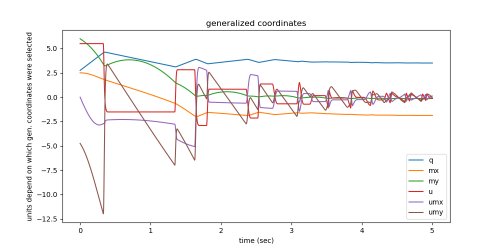
Plot the generalized coordinates you want to see.
fig, ax = plt.subplots(figsize=(10, 5))
bezeichnung = ['q', 'mx', 'my', 'u', 'umx', 'umy']
for i in (0, 1, 2, 3, 4, 5):
ax.plot(times[: resultat.shape[0]], resultat[:, i], label=bezeichnung[i])
ax.set_xlabel('time (sec)')
ax.set_ylabel('units depend on which gen. coordinates were selected')
ax.set_title('generalized coordinates')
_ = ax.legend()
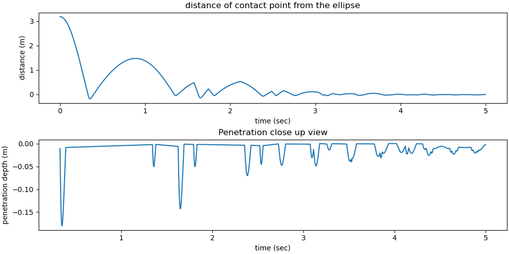
Location and distance of contact point
The distance is needed for the spring energy and the H-C hysteresis curves below.The closest distance to a possible contact point is available only during numerical integration, so they must be calculated again here. This is time consuming.
def nachrechnen():
x0 = list((-100., 100.))
kontakte = []
for i in range(schritte):
q1 = resultat[i, 0]
mx1 = resultat[i, 1]
my1 = resultat[i, 2]
TEST = []
for epsilon in np.linspace(1.e-15, 2.*np.pi, int(25/min_winkel)):
if nhat_lam(q1, epsilon, a1, b1)[1] <= 0.:
args1 = list((q1, mx1, my1, a1, b1, amplitude1, frequenz1,
epsilon))
ergebnis = root(func_x1_l1, x0, args1, method='broyden1')
x0 = ergebnis.x
x1 = x0[0]
if parallel_lam(q1, mx1, my1, x1, epsilon, a1, b1, amplitude1,
frequenz1) < min_winkel:
TEST.append((*x0, epsilon))
if len(TEST) > 0:
kontakt = min(TEST, key=lambda k: k[1])
else:
# simply attach the last 'valid' contact point data
kontakt = [kontakt[0], kontakt[1], epsilon]
kontakte.append(kontakt)
kontakte = np.array(kontakte)
if len(kontakte) != len(times):
raise Exception('something is wrong!')
return kontakte
if force_display is True:
kontakte = nachrechnen()
fig, ax = plt.subplots(2, 1, figsize=(10, 5), layout='constrained')
ax[0].plot(times, kontakte[:, 1])
ax[0].set_title('distance of contact point from the ellipse')
ax[0].set_xlabel('time (sec)')
ax[0].set_ylabel('distance (m)')
test1 = []
test2 = []
for i in range(len(kontakte)):
if kontakte[i, 1] <= 0.:
test1.append(times[i])
test2.append(kontakte[i, 1])
ax[1].plot(test1, test2)
ax[1].set_title('Penetration close up view')
ax[1].set_xlabel('time (sec)')
_ = ax[1].set_ylabel('penetration depth (m)')
print((f'There are {len(test1)} points where penetration takes place, '
f'{(len(test1)/schritte * 100):.3f} % of total points'))
else:
pass
There are 993 points where penetration takes place, 34.965 % of total points
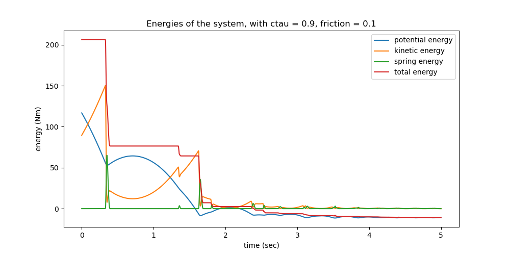
Energies of the system
For \(c_{\tau} = 1\) and reibung = 0.0, the total energy should be constant, else it should drop. The spring energy is wrong sometimes. Maybe this is the reason: The penetration depths are calculated again, see above. This may not give the same values as the ones used during the integration.
show_spring = True
kin_np = np.empty(schritte)
pot_np = np.empty(schritte)
spring_np = np.empty(schritte)
total_np = np.empty(schritte)
total1_np = np.empty(schritte)
for i in range(schritte):
if force_display is True:
pL_vals[1] = kontakte[i, 1]
pL_vals[2] = kontakte[i, 2]
kin_np[i] = kin_lam(*[resultat[i, j] for j in range(resultat.shape[1])],
*pL_vals)
pot_np[i] = pot_lam(*[resultat[i, j] for j in range(resultat.shape[1])],
*pL_vals)
spring_np[i] = spring_lam(*[resultat[i, j]
for j in range(resultat.shape[1])], *pL_vals)
total_np[i] = kin_np[i] + pot_np[i] + spring_np[i]
total1_np[i] = kin_np[i] + pot_np[i]
fig, ax = plt.subplots(figsize=(10, 5))
if show_spring is True and force_display is True:
ax.plot(times, pot_np, label='potential energy')
ax.plot(times, kin_np, label='kinetic energy')
ax.plot(times, spring_np, label='spring energy')
ax.plot(times, total_np, label='total energy')
else:
ax.plot(times, pot_np, label='potential energy')
ax.plot(times, kin_np, label='kinetic energy')
ax.plot(times, total1_np, label='total energy')
ax.set_xlabel('time (sec)')
ax.set_ylabel("energy (Nm)")
ax.set_title(f'Energies of the system, with ctau = {ctau1}, '
f'friction = {reibung1}')
_ = ax.legend()
total_max = np.max(total_np)
total_min = np.min(total_np)
if ctau1 == 1.:
print(('max deviation of total energy from being constant is {:.2e} % of '
'max total energy'.format((total_max - total_min)/total_max * 100)))
Hunt-Crossley Hysteresis Curve
The H-C model of impact, when the force is plotted against the penetration depth should give a hysterisis curve. This is done here. The black numbers on the graph give the approximate time of the ‘process’ of the impact. \(i_0\) is used to get the approximate \(\dot \rho^{(-)}\), the speed right before the impact takes place, needed for the H-C model. As the contact force depends on the location of the contact point and on the rotation of the ellipse, via \(R_1\) and \(R_2\), the curves are not necessarily nested as in other examples.
if force_display is True:
# Select approx. how many times should be printed on the graph
# select, which hystersis curves you want to see
# =======================
zeitpunkte = 5
ansehen = [0, 2, 4]
# =======================
ansehen = sorted(ansehen)
fHC_betrag_lam = sm.lambdify(qL + pL, fHC_betrag, cse=True)
HC_kraft = []
HC_displ = []
HC_times = []
zaehler = 0
i0 = 0
for i in range(resultat.shape[0]):
abstand = -kontakte[i, 1]
if abstand < 0.:
i0 = i+1
if abstand >= 0. and i0 == i:
pL_vals[1] = kontakte[i, 1]
pL_vals[2] = kontakte[i, 2]
pL_vals[-1] = rhodt_lam(*[resultat[i, j] for j in (0, 3, 4, 5)],
a1, b1, pL_vals[2])
# Put a marker, so later the individual hysteresis curves may be separated
HC_kraft.append('X')
HC_displ.append('X')
HC_times.append('X')
if abstand >= 0.:
pL_vals[1] = kontakte[i, 1]
pL_vals[2] = kontakte[i, 2]
kraft0 = fHC_betrag_lam(*[resultat[i, j]
for j in range(resultat.shape[1])],
*pL_vals)
HC_displ.append(abstand)
HC_kraft.append(kraft0)
HC_times.append((zaehler, times[i]))
zaehler += 1
# separate the lists at the marker. Found it in stack overflow
HC_kraft1 = [list(y) for x, y in itt.groupby(HC_kraft, lambda z: z == 'X')
if not x]
HC_displ1 = [list(y) for x, y in itt.groupby(HC_displ, lambda z: z == 'X')
if not x]
HC_times1 = [list(y) for x, y in itt.groupby(HC_times, lambda z: z == 'X')
if not x]
# this is to ajust the index further down
abzug = np.cumsum([0] + [len(HC_times1[i]) for i in range(len(HC_times1))])
if np.any(np.array(ansehen) > len(HC_kraft1) - 1):
raise Exception((f'You want to see a curve which does not exist. '
f'There are only {len(HC_kraft1)} curves'))
# This is to asign colors of 'plasma' to the curves.
Test = matplotlib.colors.Normalize(0, len(HC_kraft1))
Farbe = matplotlib.cm.ScalarMappable(Test, cmap='plasma')
# color of the starting position
farben = [Farbe.to_rgba(l1) for l1 in range(len(HC_kraft1))]
fig, ax = plt.subplots(figsize=(10, 5))
for i, j in enumerate(ansehen):
ax.plot(HC_displ1[j], HC_kraft1[j], color=farben[j])
ax.set_xlabel('penetration depth (m)')
ax.set_ylabel('contact force (N)')
ax.set_title((f'hysteresis curves of the {ansehen}th impacts of the '
f'ellipse with the street, ctau = {ctau1}'))
reduction = max(1, int(len(HC_times1[j])/zeitpunkte))
for k in range(len(HC_times1[j])):
if k % reduction == 0:
coord = HC_times1[j][k][0] - abzug[j]
ax.text(HC_displ1[j][coord], HC_kraft1[j][coord],
f'{HC_times1[j][k][1]:.3f}', color="black")
else:
pass
![hysteresis curves of the [0, 2, 4]th impacts of the ellipse with the street, ctau = 0.9](../_images/sphx_glr_plot_ellipse_bouncing_on_street_HC_theory_005.png)
Animation
The dotted lines show the ‘closest’ contact point, that is the point where the ellipse would touch the street if it were ‘blown up’ to just touch the street at this specific point in time. (if force_display = False the contact points were not calculated, and cannot be shown.)
schrittzahl = 100
faktor = max(1, int(resultat.shape[0] / schrittzahl))
resultat1 = []
times1 = []
kontakte1 = []
for i in range(resultat.shape[0]):
if i % faktor == 0:
resultat1.append(resultat[i, :])
times1.append(times[i])
schritte1 = len(times1)
if force_display is False:
kontakte1 = [[1000., 1000.] for i in range(schritte1)]
else:
kontakte1 = []
for i in range(resultat.shape[0]):
if i % faktor == 0:
kontakte1.append(kontakte[i])
print('points in time considered: ', len(times1))
resultat1 = np.array(resultat1)
times1 = np.array(times1)
kontakte1 = np.array(kontakte1)
Dmcx = np.array([resultat1[i, 1] for i in range(resultat1.shape[0])])
Dmcy = np.array([resultat1[i, 2] for i in range(resultat1.shape[0])])
Po_lam = sm.lambdify(qL + pL, [me.dot(Po.pos_from(P0), uv)
for uv in (N.x, N.y)])
Po_np = np.array([Po_lam(*[resultat1[i, j] for j in range(6)], *pL_vals)
for i in range(schritte1)])
# needed to give the picture the right size.
xmin = np.min(Dmcx)
xmax = np.max(Dmcx)
ymin = np.min(Dmcy)
ymax = np.max(Dmcy)
# Data to draw the uneven street
cc = max(a1, b1)
strassex = np.linspace(xmin - 1.*cc, xmax + 1.*cc, schritte1)
strassey = [gesamt_lam(strassex[i], amplitude1, frequenz1)
for i in range(schritte1)]
if u1 > 0.:
wohin = 'left'
else:
wohin = 'right'
def animate_pendulum(times, x1, y1, z1):
fig, ax = plt.subplots(figsize=(8, 8), subplot_kw={'aspect': 'equal'})
ax.axis('on')
ax.set_xlim(xmin - 1.*cc, xmax + 1.*cc)
ax.set_ylim(ymin - 1.*cc, ymax + 1.*cc)
ax.plot(strassex, strassey)
# center of the ellipse
line1, = ax.plot([], [], 'o-', lw=0.5)
# particle on the ellipse
line2, = ax.plot([], [], 'o', color="black")
line3 = ax.axvline(kontakte1[0, 0], linestyle='--', color='blue')
line4 = ax.axhline(gesamt_lam(kontakte1[0, 0], amplitude1, frequenz1),
linestyle='--', color='blue')
elli = patches.Ellipse((x1[0], y1[0]), width=2.*a1, height=2.*b1,
angle=np.rad2deg(resultat[0, 0]), zorder=1,
fill=True, color='red', ec='black')
ax.add_patch(elli)
def animate(i):
message = (f'running time {times[i]:.2f} sec \n Initial speed is '
f'{np.abs(u1):.2f} radians/sec to the {wohin}'
f'\n The black dot is the particle \n'
f'The blue dotted crosshair give the closest potential \n '
f'contact point and then the actual contact point')
ax.set_title(message, fontsize=12)
ax.set_xlabel('X direction', fontsize=12)
ax.set_ylabel('Y direction', fontsize=12)
elli.set_center((x1[i], y1[i]))
elli.set_angle(np.rad2deg(resultat1[i, 0]))
line1.set_data([x1[i]], [y1[i]])
line2.set_data([z1[i, 0]], [z1[i, 1]])
line3.set_xdata([[kontakte1[i, 0]], [kontakte1[i, 0]]])
wert = gesamt_lam(kontakte1[i, 0], amplitude1, frequenz1)
line4.set_ydata([wert, wert])
return line1, line2, line3, line4,
anim = animation.FuncAnimation(fig, animate, frames=schritte1,
interval=1250*np.max(times1) / schritte1,
blit=True)
return anim
anim = animate_pendulum(times1, Dmcx, Dmcy, Po_np)
plt.show()
points in time considered: 102
Total running time of the script: (14 minutes 43.252 seconds)