Two Balls Rolling on an Uneven Street

Objectives

• Show how to use Kane’s equations of motion in a somewhat nontrivial situation.

• Show how to use Hunt-Crossley’s theory of impact.

• Show how to use a no slip condition in a somewhat nontrivial situation.

Description

Two uniform, solid balls with radius r are running on an uneven street without slipping. The balls are not allowed to jump, but are in contact with the street at all times. The reaction forces to hold one of them on the street without slipping are calculated. A square of vertical walls ( the positive Y direction ) surrounds the street. the four corners of the square have (X / Z) coordinates: \((-l_W, -l_W), (l_W, -l_W), (l_W, l_W), (-l_W, l_W)\). \(\textrm{wall}_0\) is the bottom horizontal wall, the rest is counted counter clockwise.

The basic shape of the street is modeled by strassen_form, the superimposed unevenness is modeled by strasse. (Strasse = Street in German)

An observer, a particle of mass \(m_o\), may be attached anywhere inside each ball.

Notes

• Even a problem like this has a mass matrix of over 100,000 operations and a force vector of over 2.1 mio operations. Difficult to imagine to set up the equations of motion by hand.

Variables / Parameters. \(i \in (1, 2)\) for the two balls

• \(q_{1i}, q_{2i}, q_{3i}\): generalized coordinates of the two balls

• \(u_{1i}, u_{2i}, u_{3i}\): angular velocities of the two balls

• \(x_i, z_i\): coordinates of the contact point of the ball with the street

• \(u_{xi}, u_{zi}\): their speeds

• \(aux_x, aux_y, aux_z, f_x, f_y, f_z\): virtual speeds and reaction forces on the center of the ball

• \(m\): mass of the ball

• \(m_o\): mass of the particle on the ball

• \(r\): radius of the ball

• \(i_{XX}, i_{YY}, i_{ZZ}\): moments of inertia of the ball

• \(\textrm{amplitude, frequenz}\): parameters for the street

• \(m_u\): friction between balls

• \(m_{uW}\): friction between balls and walls

• \(\alpha, \beta, \gamma\): give the positions of the particle relative to the center of the ball

• \(N, A_1, A_2\): inertial frame, frame fixed to ball 1, frame fixed to ball 2

• \(P_0\): point fixed in N

• \(CP_i\): contact point of ball i with the street

• \(Dmc_i\): center of the ball i

• \(m_{Dmc_i}\): position of observer of ball i

• \(rhodt_\textrm{wall}\): max speed just before collission of ball i with wall j

• \(rhodt_\textrm{max}\): max speed just before collision between the walls

• \(k_0, k_{0W}\): spring constants for the balls and the walls

• \(l_W\): distance of the walls from the center of the street

• \(c_\tau\): coefficient of restitution, see Hunt Crossley

import sympy as sm
import sympy.physics.mechanics as me
import numpy as np
from scipy.integrate import solve_ivp
from scipy.optimize import minimize, root
import matplotlib.pyplot as plt
import matplotlib as mp
mp.rcParams['animation.embed_limit'] = 2**128
from matplotlib import animation

Needed to exit a loop.

class Rausspringen(Exception):
    pass

Kane’s Equations of Motion

q11, q12, q13, q21, q22, q23 = me.dynamicsymbols('q11, q12, q13, q21, q22,'
                                                 'q23')
u11, u12, u13, u21, u22, u23 = me.dynamicsymbols('u11, u12, u13, u21, u22,'
                                                 'u23')

x1, z1, x2, z2 = me.dynamicsymbols('x1, z1, x2, z2')
ux1, uz1, ux2, uz2 = me.dynamicsymbols('ux1, uz1, ux2, uz2')

rhodtwall = [[sm.symbols('rhodtwall' + str(j) + str(i))
              for i in range(4)] for j in (1, 2)]

rhodtmax = [sm.symbols('rhodtmax' + str(i)) for i in (1, 2)]
# for the reaction forces.
auxx, auxy, auxz, fx, fy, fz = me.dynamicsymbols('auxx, auxy, auxz, fx, fy,'
                                                 'fz')


m, mo, g, r, iXX, iYY, iZZ, k0, k0W, lW, ctau, mu, muW = sm.symbols(
    'm, mo, g, r, iXX, iYY, iZZ, k0, k0W, lW, ctau, mu, muW')
amplitude, frequenz, reibung, alpha, beta, gamma, t = sm.symbols('amplitude '
                                                                 'frequenz '
                                                                 'reibung '
                                                                 'alpha beta '
                                                                 'gamma t')

N, A1, A2, A3 = sm.symbols('N, A1, A2, A3', cls=me.ReferenceFrame)
P0, CP1, CP2, Dmc1, Dmc2, m_Dmc1, m_Dmc2 = sm.symbols('P0, CP1, CP2, Dmc1, '
                                                      'Dmc2, m_Dmc1, m_Dmc2',
                                                      cls=me.Point)
P0.set_vel(N, 0)

Define the street and find its minimum osculating circle

The larger the integer rumpel is, the more uneven the street.

The radius of the ball must be smaller than the smallest osculating circle (Schmiegekreis) of the road, as it must only touch the street at exactly one point. In this 3D case, the smaller one of the two osculating circles in X and Z direction is used.

Define the rotations of the frame \(A_1, A_2\), and the contact points \(CP_1, CP_2\).

\(rot, rot_1\) are used for the kinematic equations, that is \(\frac{d}{dt}q_i = f_i(q_1, q_2, q_3, u_1, u_2, u_3, \textrm{params})\)

As the mass matrix and the force vector are large, getting the term info, such as dynamic symbols takes time. With term_info = False, this may be suppressed.

rumpel = 2  # the higher the number the more 'uneven the street'.
term_info = False  # if True, term info is displayed

x, z = sm.symbols('x, z')


def gesamt(x, z):
    strasse = sum([amplitude/j * (sm.sin(j*frequenz * x) +
                                  sm.sin(j*frequenz * z))
                   for j in range(1, rumpel)])
    strassen_form = (frequenz/2. * x)**2 + (frequenz/2. * z)**2
    return strassen_form + strasse


# osculating circles in X / Z directions.
r_max_x = ((sm.S(1.) + (gesamt(x, z).diff(x))**2)**sm.S(3/2) /
           gesamt(x, z).diff(x, 2))
r_max_z = ((sm.S(1.) + (gesamt(x, z).diff(z))**2)**sm.S(3/2) /
           gesamt(x, z).diff(z, 2))

A1.orient_body_fixed(N, (q11, q12, q13), '123')
rot11 = (A1.ang_vel_in(N))
A1.set_ang_vel(N, u11*A1.x + u12*A1.y + u13*A1.z)
rot12 = (A1.ang_vel_in(N))

A2.orient_body_fixed(N, (q21, q22, q23), '123')
rot21 = (A2.ang_vel_in(N))
A2.set_ang_vel(N, u21*A2.x + u22*A2.y + u23*A2.z)
rot22 = (A2.ang_vel_in(N))

Determine the location of the center of the ball and the speed of (subsequent!) contact points

Here it is used that the balls cannot slip on the street.

vektor is the normal to the street at point (x, z), the contact point \(C_i\). It should point ‘inwards’, hence the leading minus sign.

\(Dmc_i\) is in the direction of this normal at distance r from \(CP_i\).

As the contact points \(CP_i\) are momentarily fixed in \(A_i\), one may take v2pt_theory to determine the speed of \(Dmc_i\).

Relationship of x(t) to q(t):

Obviously, x(t) = function(q(t), gesamt(x(t), z(t)), r). When the ball is rotated through an angle \(q(t)\), the arc length is \(r \cdot q(t)\).

The arc length of a function f(k(t)) from 0 to \(x(t)\) is: \(\int_{0}^{x(t)}\sqrt{1 + \left(\frac{d}{dk}f(k(t))\right) ^2} \,dk\)

This gives the sought after relationship between \(q(t)\) and \(x(t)\): \(r \cdot (-q(t)) = \int_{0}^{x(t)} \sqrt{1 + \left(\frac{d}{dk} (gesamt(k(t), z(t))\right) ^2} \,dk\), differentiated:

• \(r \cdot (-u) = \sqrt{1 + \left(\frac{d}{dx}(gesamt(x(t), z(t))\right) ^2} \cdot \frac{d}{dt}(x(t))\), that is solved for \(\frac{d}{dt}(x(t))\):

• \(\frac{d}{dt}(x(t)) = \dfrac{-(r \cdot u)} {\sqrt{1 + \left(\frac{d}{dx}(gesamt(x(t), z(t))\right) ^2}}\)

A similar formula holds for the speed in Z direction, hence one gets

\(\frac{d}{dt}(x(t)) = \dfrac{- (u3 \cdot r)} {\sqrt{1 + \left(\frac{d}{dx}(gesamt(x(t), z(t))\right) ^2}}\)

\(\frac{d}{dt}(z(t)) = \dfrac{(u1 \cdot r)} {\sqrt{1 + \left(\frac{d}{dz}(gesamt(x(t), z(t)))\right) ^2}}\)

As speeds are vectors, they can be added to give the resultant speed.

The + / - signs are a consequence of the ‘right hand rule’ for frames. These are the sought after first order differential equations for (x(t), z(t))

# location of the contact points, where the balls touch the street
CP1.set_pos(P0, x1*N.x + gesamt(x1, z1)*N.y + z1*N.z)
CP2.set_pos(P0, x2*N.x + gesamt(x2, z2)*N.y + z2*N.z)

# first ball
vektor = -(gesamt(x1, z1).diff(x1)*N.x - N.y + gesamt(x1, z1).diff(z1)*N.z)
Dmc1.set_pos(CP1, r * vektor.normalize())
m_Dmc1.set_pos(Dmc1, r*(alpha*A1.x + beta*A1.y + gamma*A1.z))

OMEGA = A1.ang_vel_in(N)
u3_wirk = me.dot(OMEGA, N.z)
u1_wirk = me.dot(OMEGA, N.x)
rhsx1 = (-u3_wirk * r / sm.sqrt(1. + gesamt(x1, z1).diff(x1)**2))
rhsz1 = (u1_wirk * r / sm.sqrt(1. + gesamt(x1, z1).diff(z1)**2))

# second ball
vektor = -(gesamt(x2, z2).diff(x2)*N.x - N.y + gesamt(x2, z2).diff(z2)*N.z)
Dmc2.set_pos(CP2, r * vektor.normalize())
m_Dmc2.set_pos(Dmc2, r*(alpha*A2.x + beta*A2.y + gamma*A2.z))

OMEGA = A2.ang_vel_in(N)
u3_wirk = me.dot(OMEGA, N.z)
u1_wirk = me.dot(OMEGA, N.x)
rhsx2 = (-u3_wirk * r / sm.sqrt(1. + gesamt(x2, z2).diff(x2)**2))
rhsz2 = (u1_wirk * r / sm.sqrt(1. + gesamt(x2, z2).diff(z2)**2))

# this is needed at various places below
rhs_dict = {sm.Derivative(i, t): j for i, j in zip((x1, z1, x2, z2),
                                                   (rhsx1, rhsz1, rhsx2,
                                                    rhsz2))}

CP1.set_vel(N, CP1.pos_from(P0).diff(t, N).subs(rhs_dict))
CP2.set_vel(N, CP2.pos_from(P0).diff(t, N).subs(rhs_dict))

Dmc1.set_vel(N, Dmc1.pos_from(P0).diff(t, N).subs(rhs_dict) +
             auxx*N.x + auxy*N.y + auxz*N.z)
m_Dmc1.v2pt_theory(Dmc1, N, A1)

Dmc2.set_vel(N, Dmc2.pos_from(P0).diff(t, N).subs(rhs_dict))
m_Dmc2.v2pt_theory(Dmc2, N, A2)

if term_info:
    print('CP1 DS', me.find_dynamicsymbols(CP1.vel(N), reference_frame=N))
    print('vel(Dmc2) DS:', me.find_dynamicsymbols(Dmc2.vel(N),
                                                  reference_frame=N))

Function which calculates the forces of an impact between a ball and a wall

1. The impact force is on the line normal to the wall, going through the center of the ball, \(Dmc_i\). I use Hunt Crossley’s method to calculate it. It’s direction points from the wall to the ball.

2. The friction force acting on the contact point \(CP_0\) is proportional to the component of the speed of \(CP_0\) in the plane of the wall, the impact force and a friction factor \(m_{uW}\) It is equivalent to a force through \(Dmc_i\) and to a torque acting on \(A_i\), the ball fixed frame.

Note about the force during the collisions

Hunt Crossley’s method

Reference is this article https://www.sciencedirect.com/science/article/pii/S0094114X23000782

This is with dissipation during the collision, the general force is given in (63) as:

\(f_n = k_0 \cdot \rho + \chi \cdot \dot \rho\), with \(k_0\) as below, \(\rho\) the penetration, and \(\dot\rho\) the speed of the penetration. In the article it is stated, that \(n = \frac{3}{2}\) is a good choice, it is derived in Hertz’ approach. Of course, \(\rho, \dot\rho\) must be the signed magnitudes of the respective vectors.

A more realistic force is given in (64) as:

\(f_n = k_0 \cdot \rho^n + \chi \cdot \rho^n\cdot \dot \rho\), as this avoids discontinuity at the moment of impact.

Hunt and Crossley give this value for \(\chi\), see table 1:

\(\chi = \dfrac{3}{2} \cdot(1 - c_\tau) \cdot \dfrac{k_0}{\dot \rho^{(-)}}\), where

\(c_\tau = \dfrac{v_1^{(+)} - v_2^{(+)}}{v_1^{(-)} - v_2^{(-)}}\), where

\(v_i^{(-)}, v_i^{(+)}\) are the speeds of \(\textrm{body}_i\), before and after the collosion, see (45),

\(\dot\rho^{(-)}\) is the speed right at the time the impact starts.

\(c_\tau\) is an experimental factor, apparently around 0.8 for steel.

Using (64), this results in their expression for the force:

\(f_n = k_0 \cdot \rho^n \left[1 + \dfrac{3}{2} \cdot(1 - c_\tau) \cdot \dfrac{\dot\rho}{\dot\rho^{(-)}}\right]\)

with

\(\frac{R_1 \cdot R_2}{R_1 + R_2}\), where

\(\sigma_i = \frac{1 -\nu_i^2}{E_i}\), with

\(\nu_i\) = Poisson’s ratio, \(E_i\) = Young”s modulus, \(R_1, R_2\) the radii of the colliding bodies, \(\rho\) the penetration depth. All is near equations (54) and (61) of this article.

As per the article, \(n = \frac{3}{2}\) is always to be used.

spring energy = \(k_0 \cdot \int_{0}^{\rho} k^{3/2}\,dk = k_0 \cdot\frac{2}{5} \cdot \rho^{5/2}\)

I assume, the dissipated energy cannot be given in closed form, at least the article does not give one.

Note

\(c_\tau = 1.\) gives Hertz’s solution to the impact problem, also described in the article.

Friction when a ball hits a wall

This website: https://math.stackexchange.com/questions/2195047/solve-the-vector-cross-product-equation

gives: \(b = a \times x \rightarrow x = \dfrac{b \times a}{|a|^2}\)

This way, one can easily get the friction force acting on \(CP_0\) (contact point of ball with wall), without any further geometric considerations. Of course the friction force has opposite to the speed of \(C_0\).

The friction force on \(C_0\) is equivalent to a force on \(Dmc_i\) (center of the ball) and a torque on \(A_i\) (ball fixed frame)

def HC_wall(N, A1, P1, r, ctau, rhodtwall, k0W):

    FC = []
    FF = []
    TF = []
    TT = []
    for l, richtung in enumerate((N.z, -N.x, -N.z, N.x)):

        abstand = lW + me.dot(P1.pos_from(P0), richtung)
        rho = r - abstand       # positive in the ball has penetrated the wall
        CP0 = me.Point('CP0')
        CP0.set_pos(P1, -richtung)
        vCP0 = CP0.v2pt_theory(P1, N, A1)
        rhodt = me.dot(vCP0, richtung)
        rho = sm.Max(rho, sm.S(0))

        forcec = (k0W * rho**(3/2) * (1. + 3./2. * (1 - ctau) * rhodt /
                                      rhodtwall[l]) *
                  (richtung * sm.Heaviside(r - abstand, 0.)))

        friction_force = forcec.magnitude() * muW * (-CP0.vel(N))
        hilfs = CP0.pos_from(P1)
        torque = hilfs.cross(friction_force) * sm.Heaviside(r - abstand, 0.)
        forcef = (1./me.dot(hilfs, hilfs) * torque.cross(hilfs) *
                  sm.Heaviside(r - abstand, 0.))

        FC.append(forcec)
        FF.append(forcef)
        TF.append(torque)

    for i in (FC, FF, TF):
        TT.append(i)
    return TT

Calculates the forces and the torques when the two balls collide. Similar to the ideas above.

def HC_disc(N, A1, A2, P1, P2, r, ctau, rhodtmax, k0):
    '''
This function returns the forces, torques on P2, when colliding with P1.
Very similar to HC_wall above
    '''
    vektor = P2.pos_from(P1)
    richtung = vektor.normalize()
    abstand = vektor.magnitude()
    rho = 2. * r - abstand   # positive in the ball has penetrated the wall
    CP01 = me.Point('CP01')
    CP01.set_pos(P1, 0.5 * abstand * richtung)
    vCP01 = CP01.v2pt_theory(P1, N, A1)
    rhodt = me.dot(vCP01, richtung)
    rho = sm.Max(rho, sm.S(0))

    forcec = (k0 * rho**(3/2) * (1. + 3./2. * (1 - ctau) * rhodt / rhodtmax)
              * (richtung * sm.Heaviside(2. * r - abstand, 0.)))

    CP02 = me.Point('CP02')
    CP02.set_pos(P2, -0.5 * abstand * richtung)
#    vCP02 = CP02.v2pt_theory(P2, N, A2)

    friction_force = forcec.magnitude() * mu * -(CP02.vel(N) - CP01.vel(N))
    hilfs = CP02.pos_from(P2)
    torque = hilfs.cross(friction_force) * sm.Heaviside(2. * r - abstand, 0.)
    forcef = (1./me.dot(hilfs, hilfs) * torque.cross(hilfs) *
              sm.Heaviside(2. * r - abstand, 0.))

    return [forcec, forcef, torque]

Various functions needed later. The bodies must be defined here, as they are needed for the kinetic energy.

• distanzw: distance from the ball to the walls

• abstand_baelle: distance of the two balls from each other

• rhodtwall: speed right at impact. it is calculated same as rhodt in the function HC_wall

• rhodtmax: speed right before the impact of the two balls

• pot_energie: potential energy

• kin_energie: kinetic energy

• spring_energie: energy stored in the ball during collissions with the walls

I1 = me.inertia(A1, iXX, iYY, iZZ)
Body1 = me.RigidBody('Body1', Dmc1, A1, m, (I1, Dmc1))
observer1 = me.Particle('observer1', m_Dmc1, mo)

I2 = me.inertia(A2, iXX, iYY, iZZ)
Body2 = me.RigidBody('Body2', Dmc2, A2, m, (I2, Dmc2))
observer2 = me.Particle('observer2', m_Dmc2, mo)

BODY = [Body1, Body2, observer1, observer2]

subs_dict1 = {sm.Derivative(i, t): j for i, j in zip((q11, q12, q13, q21, q22,
                                                      q23),
                                                     (u11, u12, u13, u21, u22,
                                                      u23))}
energie_dict = {i: 0. for i in (auxx, auxy, auxz, fx, fy, fz)}

distanz_list = [[lW + me.dot(ball.pos_from(P0), richtung)
                 for richtung in (N.z, -N.x, -N.z, N.x)]
                for ball in (Dmc1, Dmc2)]
abstand_baelle = Dmc1.pos_from(Dmc2).magnitude()

rhodtwall_list = []
for ball, frame in zip((Dmc1, Dmc2), (A1, A2)):
    hilfs = []
    for richtung in (N.z, -N.x, -N.z, N.x):
        CP0 = me.Point('CP0')
        CP0.set_pos(ball, -richtung)
        vCP0 = CP0.v2pt_theory(ball, N, frame)
        rhodt = me.dot(vCP0, richtung).subs(energie_dict)
        hilfs.append(rhodt)
    rhodtwall_list.append(hilfs)

richtung = Dmc1.pos_from(Dmc2).normalize()
rhodtmax_list = [hilfs0 := me.dot(Dmc2.pos_from(Dmc1).diff(t, N),
                                  richtung).subs(rhs_dict), -hilfs0]
if term_info is True:
    print(me.find_dynamicsymbols(rhodtmax_list[0], reference_frame=N))

    hilfs1 = set()
    hilfs2 = set()
    hilfs3 = set()
    hilfs4 = set()
    for k in range(2):
        hilfs1 = hilfs1.union(*[me.find_dynamicsymbols(distanz_list[k][l])
                                for l in range(4)])
        hilfs2 = hilfs2.union(*[distanz_list[k][l].free_symbols
                                for l in range(4)])
        hilfs3 = hilfs3.union(*[me.find_dynamicsymbols(rhodtwall_list[k][l])
                                for l in range(4)])
        hilfs4 = hilfs4.union(*[rhodtwall_list[k][l].free_symbols
                                for l in range(4)])
    print('distanz_list DS', hilfs1)
    print('distanz_list FS', hilfs2, '\n')
    print('rhodtwall_list DS', hilfs3)
    print('rhodtwall_list FS', hilfs4, '\n')

pot_energie = ((m * g * me.dot(Dmc1.pos_from(P0), N.y) + mo * g *
               me.dot(m_Dmc1.pos_from(P0), N.y) + m * g *
               me.dot(Dmc2.pos_from(P0), N.y) + mo * g *
               me.dot(m_Dmc2.pos_from(P0), N.y)).subs(rhs_dict).
               subs(energie_dict))

kin_energie = sum([koerper.kinetic_energy(N).subs(rhs_dict).subs(energie_dict)
                   for koerper in BODY])

spring_energie = 0.
# contribution of the walls
for k in range(2):
    for i in range(4):
        rho = sm.Max(r - distanz_list[k][i], 0.)
        spring_energie += (2./5. * k0W * rho**(5/2) *
                           sm.Heaviside(r - distanz_list[k][i], 0.))
# contribution of the two balls colliding
rho = sm.Max(2. * r - Dmc1.pos_from(Dmc2).magnitude(), 0.)
spring_energie += (2./5. * k0 * rho**(5/2) *
                   sm.Heaviside(2. * r - Dmc1.pos_from(Dmc2).magnitude(),
                                0.))

if term_info:
    print('pot energy DS', me.find_dynamicsymbols(pot_energie), '\n')
    print('kin energy DS', me.find_dynamicsymbols(kin_energie), '\n')
    print('spring energy DS', me.find_dynamicsymbols(spring_energie), '\n')
# various points
CP1_pos = [(me.dot(CP1.pos_from(P0), uv)).subs(rhs_dict) for uv in N]
Dmc1_pos = [(me.dot(Dmc1.pos_from(P0), uv)).subs(rhs_dict) for uv in N]
m_Dmc1_pos = [(me.dot(m_Dmc1.pos_from(P0), uv)).subs(rhs_dict) for uv in N]

CP2_pos = [(me.dot(CP2.pos_from(P0), uv)).subs(rhs_dict) for uv in N]
Dmc2_pos = [(me.dot(Dmc2.pos_from(P0), uv)).subs(rhs_dict) for uv in N]
m_Dmc2_pos = [(me.dot(m_Dmc2.pos_from(P0), uv)).subs(rhs_dict) for uv in N]

Set the forces and torques for Kane’s equations.

FL = [(Dmc1, -m*g*N.y), (m_Dmc1, -mo*g*N.y), (Dmc1, fx*N.x + fy*N.y + fz*N.z)]
FL.append((Dmc2, -m*g*N.y))
FL.append((m_Dmc2, -mo*g*N.y))

# collisions with the walls
zaehler = 0
for ball, frame in zip((Dmc1, Dmc2), (A1, A2)):
    for i in range(4):
        FL.append((ball, HC_wall(N, frame, ball, r, ctau, rhodtwall[zaehler],
                                 k0W)[0][i]))  # impact force
        FL.append((ball, HC_wall(N, frame, ball, r, ctau, rhodtwall[zaehler],
                                 k0W)[1][i]))  # force on Dmc, due to friction
        FL.append((frame, HC_wall(N, frame, ball, r, ctau, rhodtwall[zaehler],
                                  k0W)[2][i]))  # torque on ball, friction
    zaehler += 1

# collisions of the two balls
FL.append((Dmc1, HC_disc(N, A2, A1, Dmc2, Dmc1, r, ctau, rhodtmax[0], k0)[0]))
FL.append((Dmc1, HC_disc(N, A2, A1, Dmc2, Dmc1, r, ctau, rhodtmax[0], k0)[1]))
FL.append((A1, HC_disc(N, A2, A1, Dmc2, Dmc1, r, ctau, rhodtmax[0], k0)[2]))

FL.append((Dmc2, HC_disc(N, A1, A2, Dmc1, Dmc2, r, ctau, rhodtmax[1], k0)[0]))
FL.append((Dmc2, HC_disc(N, A1, A2, Dmc1, Dmc2, r, ctau, rhodtmax[1], k0)[1]))
FL.append((A2, HC_disc(N, A1, A2, Dmc1, Dmc2, r, ctau, rhodtmax[1], k0)[2]))

Kane’s equations of motion

The formalism to set up Kane’s equations.

As \(Dmc_1\) has a real speed and virtual speeds for the reaction forces, the reaction forces appear in the force vector. As they do no work, they are set to zero.

One needs to numerically solve the first order differential equations for \((x_1(t), z_1(t), x_2(t), z_2(t))\), so the right hand sides are added at the bottom of the force vector. The mass matrix needs to be enlarged accordingly.

kd = [me.dot(rot11 - rot12, uv) for uv in A1] + [me.dot(rot21 - rot22, uv)
                                                 for uv in A2]

q = [q11, q12, q13, q21, q22, q23]
u = [u11, u12, u13, u21, u22, u23]
aux = [auxx, auxy, auxz]

# Setting up Kane's equations
KM = me.KanesMethod(N, q_ind=q, u_ind=u, kd_eqs=kd, u_auxiliary=aux)
(fr, frstar) = KM.kanes_equations(BODY, FL)
MM1 = KM.mass_matrix_full
force1 = KM.forcing_full.subs({fx: 0., fy: 0., fz: 0.})

# add the rhsx1, etc at the bottom of the force vector
force = ((sm.Matrix.vstack(force1, sm.Matrix([rhsx1, rhsz1, rhsx2, rhsz2]))).
         subs(rhs_dict)).subs({i: 0. for i in aux})
if term_info:
    print('force DS', me.find_dynamicsymbols(force))
    print('force free symbols', force.free_symbols)
print(f'force has {sm.count_ops(force):,} operations')

# Enlarge MM properly
MM2 = sm.Matrix.hstack(MM1, sm.zeros(12, 4))
hilfs = sm.Matrix.hstack(sm.zeros(4, 12), sm.eye(4))
MM = sm.Matrix.vstack(MM2, hilfs)
if term_info:
    print('MM DS', me.find_dynamicsymbols(MM))
    print('MM free symbols', MM.free_symbols)
print(f'MM has {sm.count_ops(MM):,} operations')

force has 2,167,210 operations
MM has 105,296 operations

Reaction Forces

The function to get the reaction forces is determined. This function (of course!) needs the accelerations of points, hence values of \(rhs = MM^{-1} * force\) are needed. While one can get rhs symbolically, it probably HUGE. So, it is calculated numerically further down. RHS are just subs

RHS = [sm.symbols('rhs' + str(i)) for i in range(force.shape[0])]
eingepraegt_dict = {sm.Derivative(i, t): RHS[j] for j, i in enumerate(q + u)}
eingepraegt = ((((KM.auxiliary_eqs).subs(eingepraegt_dict)).
                subs(rhs_dict)).subs({i: 0. for i in aux}))
if term_info:
    print('eingepraegt DS', me.find_dynamicsymbols(eingepraegt))
    print('eingepraegt free symbols', eingepraegt.free_symbols)
print(f'eingepraegt has {sm.count_ops(eingepraegt):,} operations')

eingepraegt has 237,857 operations

Lambdification

pL = [m, mo, g, r, iXX, iYY, iZZ, amplitude, frequenz] + \
    [ctau, k0, k0W, lW, mu, muW] + [alpha, beta, gamma] + \
    [rhodtwall] + [rhodtmax]
pL1 = [r, lW, amplitude, frequenz]

qL = q + u + [x1, z1, x2, z2]
F = [fx, fy, fz]

MM_lam = sm.lambdify(qL + pL, MM, cse=True)
force_lam = sm.lambdify(qL + pL, force, cse=True)

CP1_pos_lam = sm.lambdify(qL + pL, CP1_pos, cse=True)
Dmc1_pos_lam = sm.lambdify(qL + pL, Dmc1_pos, cse=True)
m_Dmc1_pos_lam = sm.lambdify(qL + pL, m_Dmc1_pos, cse=True)

CP2_pos_lam = sm.lambdify(qL + pL, CP2_pos, cse=True)
Dmc2_pos_lam = sm.lambdify(qL + pL, Dmc2_pos, cse=True)
m_Dmc2_pos_lam = sm.lambdify(qL + pL, m_Dmc2_pos, cse=True)

gesamt1 = gesamt(x, z)
gesamt_lam = sm.lambdify([x, z] + [amplitude, frequenz], gesamt1, cse=True)

pot_lam = sm.lambdify(qL + pL, pot_energie, cse=True)
kin_lam = sm.lambdify(qL + pL, kin_energie, cse=True)
spring_lam = sm.lambdify(qL + pL, spring_energie, cse=True)

distanz_list_lam = sm.lambdify(qL + pL1, distanz_list, cse=True)
abstand_baelle_lam = sm.lambdify([x1, z1, x2, z2] + pL1, abstand_baelle,
                                 cse=True)

rhodtwall_list_lam = sm.lambdify(qL + pL1, rhodtwall_list, cse=True)
rhodtmax_list_lam = sm.lambdify(qL + pL1, rhodtmax_list, cse=True)

eingepraegt_lam = sm.lambdify(F + qL + pL + RHS, eingepraegt, cse=True)

r_max_lam = sm.lambdify([x, z] + pL1, [r_max_x, r_max_z], cse=True)

Numerical Integration

Input parameters / initial values of the coordinates and speeds. While it makes sense to name them similarly to the symbols / dynamic symbols used in setting up Kane’s equations, avoid the same name: the symbols will be overwritten, with unintended consequences.

The larger \(\textrm{frequenz}_1\) and the larger rumpel, the smaller the minimum osculating circle.

• \(m_1\) mass of the ball

• \(m_{o1}\) mass of observer

• \(r_1\) radius of ball

• \(lW_1\) length of the street

• \(c_\tau\) coefficient needed for the Hunt Crossley method of impact.

• \(\mu_1\) friction between ball and street

• \(\mu_W\) friction between ball and wall

• \(\alpha_1, \beta_1, \gamma_1\) location of observer relative to Dmc

• \(\textrm{amplitude}_1, \textrm{frequenz}_1\) define the street

• \(q_{110}, q_{120}, q_{130}, q_{210}, q_{220}, q_{230}\) initial values of the coordinates

• \(u_{110}, u_{120}, u_{130}, u_{210}, u_{220}, u_{230}\) initial values of the speeds

• \(x_{10}, z_{10}, x_{20}, z_{20}\) initial location of the contact point

• intervall: running time of the integration is in [0., intervall]

• schritte: solve_ivp returns the values evenly spaced in [0., intervall]

An exception is raised, if the observer was put outside the ball.

max_step = 0.01

m1 = 1.e0
mo1 = 1.e-1
r1 = 1.
lW1 = 5.
ctau1 = 0.9
mu1 = 0.01
muW1 = 0.01
amplitude1 = 2.
frequenz1 = 0.2

alpha1, beta1, gamma1 = 0., 0.8, 0.

q110, q120, q130, q210, q220, q230 = 0., 0., 0., 0., 0., 0.

intervall = 12.5

np.random.seed(42)  # for reproducibility
# set initial angular velocities randomly
u110, u120, u130, u210, u220, u230 = np.random.choice(
    np.linspace(-10, 10, 100), size=6)

print([f'{j} = {i:.2f} rad/sec  ' for j, i in zip(('u11', 'u12', 'u13',
                                                   'u21', 'u22', 'u23'),
                                                  (u110, u120, u130, u210,
                                                   u220, u230))], '\n')


# find feasible starting locations for the two balls
np.random.seed(42)  # for reproducibility
zaehler = 0
while zaehler <= 100:
    zaehler += 1
    try:
        x10, z10, x20, z20 = np.random.choice(np.linspace(-lW1 + 2.*r1, lW1
                                                          - 2.*r1, 100),
                                              size=4, replace=False)
        if (abstand_baelle_lam(x10, z10, x20, z20, r1, lW1, amplitude1,
                               frequenz1) > 3. * r1):
            raise Rausspringen()
    except Rausspringen:
        break

if zaehler <= 100:
    print(f'it took {zaehler} rounds to get valid initial conditions')
    print((f'balls are located at ({x10:.2f}/{z10:.2f}) and at '
           f'({x20:.2f}/{z20:.2f}) respectively', '\n'))
else:
    raise Exception(' no good location for discs found, make lW0 larger.')

schritte = int(intervall * 300.)
if alpha1**2 + beta1**2 + gamma1**2 >= 1.:
    raise Exception('center of mass outside of the ball')

rhodtwall1 = [[1. for _ in range(4)] for _ in range(2)]
rhodtmax1 = [1., -1.]

# Calculate k01 and k0W1
nu = 0.28  # Poisson's ratio, from the internet
# units: N/m^2, Young's modulus from the internet, around 2e11 for steel
EY = 2.e3
sigma = (1 - nu**2) / EY
k01 = 4. / (3. * (sigma + sigma)) * np.sqrt(r1 / 2.)
k0W1 = 4. / (3. * (sigma + sigma)) * np.sqrt(r1)


iXXe = 2. / 5. * m1 * r1**2

pL_vals = [m1, mo1, 9.8, r1, iXXe, iXXe, iXXe, amplitude1, frequenz1, ctau1,
           k01, k0W1,
           lW1, mu1, muW1, alpha1, beta1, gamma1] + [rhodtwall1] + [rhodtmax1]
pL1_vals = [r1, lW1, amplitude1, frequenz1]

print('pL_vals', pL_vals, '\n')

y0 = [q110, q120, q130, q210, q220, q230] + \
    [u110, u120, u130, u210, u220, u230] + [x10, z10, x20, z20]

if frequenz1 > 0.:
    # find the smallest osculating radius, given strasse, amplitude, frequenz
    def func1(x, args):
        # just needed to get the arguments matching for minimuze
        return np.abs(r_max_lam(*x, *args)[0])

    def func2(x, args):
        # just needed to get the arguments matching for minimuze
        return np.abs(r_max_lam(*x, *args)[1])

    x0 = (0.1, 0.1)      # initial guess
    minimal1 = minimize(func1, x0, pL1_vals)
    minimal2 = minimize(func2, x0, pL1_vals)

    minimal = min(minimal1.get('fun'), minimal2.get('fun'))

    if pL_vals[3] < minimal:
        print(f'selected radius = {pL_vals[3]} is less than minimally '
              f'admissible radius = {minimal:.2f}, hence o.k. \n')
    else:
        print(f'selected radius {pL_vals[3]} is larger than admissible '
              f'radius {minimal:.2f}, hence NOT o.k. \n')
        raise Exception('Radius of ball is too large')
else:
    print('Street is flat')

times = np.linspace(0, intervall, schritte)


def gradient(t, y, args):

    # get the speed of the balls right before it hit a wall
    for ball in range(2):
        for wand in range(4):
            if 0 < r1 - distanz_list_lam(*y, *pL1_vals)[ball][wand] <= 0.03:
                args[-2][ball][wand] = rhodtwall_list_lam(
                    *y, *pL1_vals)[ball][wand]
    if (0. < 2. * r1 - abstand_baelle_lam(y[-4], y[-3], y[-2], y[-1],
                                          *pL1_vals) <= 0.03):
        args[-1] = rhodtmax_list_lam(*y, *pL1_vals)

    sol = np.linalg.solve(MM_lam(*y, *pL_vals), force_lam(*y, *pL_vals))
    return np.array(sol).T[0]


t_span = (0., intervall)
resultat1 = solve_ivp(gradient, t_span, y0, t_eval=times, args=(pL_vals,),
                      method='BDF', max_step=max_step, atol=1.e-6, rtol=1.e-6)
resultat = resultat1.y.T

print(resultat1.message)
if resultat1.status == -1:
    raise Exception()
print('resultat shape', resultat.shape, '\n')

print((f"To numerically integrate an intervall of {intervall} sec the "
       f"routine made {resultat1.nfev} function calls"))

['u11 = 0.30 rad/sec  ', 'u12 = 8.59 rad/sec  ', 'u13 = -7.17 rad/sec  ', 'u21 = 4.34 rad/sec  ', 'u22 = 2.12 rad/sec  ', 'u23 = -5.96 rad/sec  ']

it took 3 rounds to get valid initial conditions
('balls are located at (-0.09/-1.30) and at (2.15/2.03) respectively', '\n')
pL_vals [1.0, 0.1, 9.8, 1.0, 0.4, 0.4, 0.4, 2.0, 0.2, 0.9, np.float64(1023.0132829666487), np.float64(1446.7592592592594), 5.0, 0.01, 0.01, 0.0, 0.8, 0.0, [[1.0, 1.0, 1.0, 1.0], [1.0, 1.0, 1.0, 1.0]], [1.0, -1.0]]

selected radius = 1.0 is less than minimally admissible radius = 10.19, hence o.k.

The solver successfully reached the end of the integration interval.
resultat shape (3750, 16)

To numerically integrate an intervall of 12.5 sec the routine made 8071 function calls

Plot whatever generalized coordinates you want to see

bezeichnung = ['q11', 'q12', 'q13', 'q21', 'q22', 'q23',
               'u11', 'u12', 'u13', 'u21', 'u22', 'u23',
               'x1', 'z1', 'x2', 'z2']
fig, ax = plt.subplots(figsize=(10, 5))
for i in (6, 10, 12, 13, 14, 15):
    ax.plot(times, resultat[:, i], label=bezeichnung[i])
ax.set_title('Generalized coordinates')
_ = ax.legend()

Draw the hysteresis curves of the impacts of the balls and of the balls with the walls. The red numbers on the graphs indicate the times during which the impact takes place. Only walls where impacts have taken place are shown.

HC_kraft = []
HC_displ = []
HC_times = []
zaehler = 0
i0 = 0
for i in range(resultat.shape[0]):
    abstand = 2. * r1 - abstand_baelle_lam(*[resultat[i, j]
                                             for j in range(-4, 0)], *pL1_vals)
    if abstand < 0.:
        i0 = i+1

    if abstand >= 0. and i0 == i:
        walldt = rhodtmax_list_lam(*[resultat[i, j]
                                     for j in range(resultat.shape[1])],
                                   *pL1_vals)[0]
    if abstand >= 0.:
        rhodt = rhodtmax_list_lam(*[resultat[i, j]
                                    for j in range(resultat.shape[1])],
                                  *pL1_vals)[0]
        kraft0 = (k01 * abstand**(3/2) * (1. + 3./2. * (1 - ctau1) *
                                          rhodt/walldt))
        HC_displ.append(abstand)
        HC_kraft.append(kraft0)
        HC_times.append((zaehler, times[i]))
        zaehler += 1

HC_displ = np.array(HC_displ)
HC_kraft = np.array(HC_kraft)
# plot only, if there were collisions with a wall.
if len(HC_displ) != 0:
    fig, ax = plt.subplots(figsize=(10, 5))
    ax.plot(HC_displ, HC_kraft, color='green')
    ax.set_xlabel('penetration depth (m)')
    ax.set_ylabel('contact force (Nm)')
    ax.set_title((f'hysteresis curves of successive impacts of the ball_1 '
                  f'with ball_2, ctau = {ctau1}, mu = {mu1}'))

    zeitpunkte = 10
    reduction = max(1, int(len(HC_times)/zeitpunkte))
    for k in range(len(HC_times)):
        if k % reduction == 0:
            coord = HC_times[k][0]
            ax.text(HC_displ[coord], HC_kraft[coord], f'{HC_times[k][1]:.2f}',
                    color="red")

HC_displ_list = []
HC_kraft_list = []
HC_times_list = []
index_list = []

for ball in range(2):
    for wall in range(4):

        HC_kraft = []
        HC_displ = []
        HC_times = []
        zaehler = 0
        i0 = 0
        for i in range(resultat.shape[0]):
            abstand = r1 - distanz_list_lam(*[resultat[i, j]
                                              for j in
                                              range(resultat.shape[1])],
                                            *pL1_vals)[ball][wall]
            if abstand < 0.:
                i0 = i+1

            if abstand >= 0. and i0 == i:
                walldt = rhodtwall_list_lam(*[resultat[i, j]
                                              for j in
                                              range(resultat.shape[1])],
                                            *pL1_vals)[ball][wall]
            if abstand >= 0.:
                rhodt = rhodtwall_list_lam(*[resultat[i, j]
                                             for j in
                                             range(resultat.shape[1])],
                                           *pL1_vals)[ball][wall]
                kraft0 = (k0W1 * abstand**(3/2) * (1. + 3./2. * (1 - ctau1) *
                                                   rhodt/walldt))
                HC_displ.append(abstand)
                HC_kraft.append(kraft0)
                HC_times.append((zaehler, times[i]))
                zaehler += 1

        HC_displ = np.array(HC_displ)
        HC_kraft = np.array(HC_kraft)
        # print only, if there were collisions with a wall.
        if len(HC_displ) != 0:
            HC_displ_list.append(HC_displ)
            HC_kraft_list.append(HC_kraft)
            HC_times_list.append(HC_times)
            index_list.append((ball, wall))

plots = len(index_list)
fig, ax = plt.subplots(plots, 1, figsize=(10, 5*plots), layout='constrained')
for i, (ball, wall) in enumerate(index_list):
    ax[i].plot(HC_displ_list[i], HC_kraft_list[i])
    ax[i].set_xlabel('penetration depth (m)')
    ax[i].set_ylabel('contact force (Nm)')
    ax[i].set_title((f'hysteresis curves of successive impacts of the '
                     f' ball_{ball+1} with wall_{wall}, ctau = {ctau1}, '
                     f'muW = {muW1}'))

    zeitpunkte = 20
    reduction = max(1, int(len(HC_times_list[i])/zeitpunkte))
    for k in range(len(HC_times_list[i])):
        if k % reduction == 0:
            coord = HC_times_list[i][k][0]
            ax[i].text(HC_displ_list[i][coord], HC_kraft_list[i][coord],
                       f'{HC_times_list[i][k][1]:.2f}', color="red")

Plot the energies of the ball. Absent any friction, that is \(\mu, \mu_W = 0.\) and \(c_\tau = 1.\) the total energy should be constant. Otherwise it should go down in steps, being constant between any impacts.

pot_np = np.empty(schritte)
kin_np = np.empty(schritte)
spring_np = np.empty(schritte)
total_np = np.empty(schritte)
for l in range(schritte):
    pot_np[l] = pot_lam(*[resultat[l, j] for j in range(resultat.shape[1])],
                        *pL_vals)
    kin_np[l] = kin_lam(*[resultat[l, j] for j in range(resultat.shape[1])],
                        *pL_vals)
    spring_np[l] = spring_lam(*[resultat[l, j]
                                for j in range(resultat.shape[1])], *pL_vals)
    total_np[l] = pot_np[l] + kin_np[l] + spring_np[l]

if ctau1 == 1. and muW1 == 0. and mu1 == 0.:
    fehler = ((x111 := max(total_np)) - min(total_np)) / x111 * 100.
    print((f'max deviation from total energy = constant is {fehler:.2e} %  '
           f'of max total energy'))
fig, ax = plt.subplots(figsize=(10, 5))
ax.plot(times, kin_np, label='kin energy')
ax.plot(times, pot_np, label='pot energy')
ax.plot(times, spring_np, label='spring energy')
ax.plot(times, total_np, label='total energy')
ax.set_title((f'Energy of the system where mu = {mu1}, muW = {muW1}, '
              f'ctau = {ctau1}'))
_ = ax.legend()

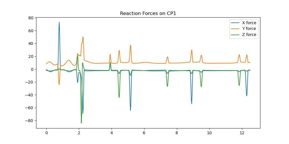
Reaction Forces

Only calculated for one ball, the second ball surely will look similar. First the rhs is calculated numerically, then eingepraegt = 0. is solved numerically for the reaction forces, then they are plotted. As there are many points in time, this may take a long time to calculate. To reduce the time, only around zeitpunkte number of points in time are considered.

times2 = []
resultat2 = []

zeitpunkte = 500

reduction = max(1, int(len(times)/zeitpunkte))

for i in range(len(times)):
    if i % reduction == 0:
        times2.append(times[i])
        resultat2.append(resultat[i])

schritte2 = len(times2)
resultat2 = np.array(resultat2)
times2 = np.array(times2)
print('number of points considered:', len(times2))

# RHS calculated numerically, too large to do it symbolically.
# Needed for reaction forces.
RHS1 = np.zeros((schritte2, resultat2.shape[1]))
for i in range(schritte2):
    RHS1[i, :] = (np.linalg.solve(MM_lam(*[resultat2[i, j] for j in
                                           range(resultat2.shape[1])],
                                         *pL_vals),
                                  force_lam(*[resultat2[i, j]
                                              for j in
                                              range(resultat2.shape[1])],
                                            *pL_vals)).
                  reshape(resultat2.shape[1]))

print('RHS1 shape', RHS1.shape)


# calculate implied forces numerically
def func(x, *args):
    # just serves to 'modify' the arguments for fsolve.
    return eingepraegt_lam(*x, *args).reshape(3)


kraftx = np.zeros(schritte2)
krafty = np.zeros(schritte2)
kraftz = np.zeros(schritte2)
x0 = tuple((1., 1., 1.))   # initial guess

for i in range(schritte2):
    for _ in range(2):
        y0 = [resultat2[i, j] for j in range(resultat2.shape[1])]
        rhs = [RHS1[i, j] for j in range(16)]
        args = tuple(y0 + pL_vals + rhs)
        A = root(func, x0, args=args)
        A = A.x  # get the solution from the root object
        x0 = tuple(A)  # improved guess. Should speed up convergence.
    kraftx[i] = A[0]
    krafty[i] = A[1]
    kraftz[i] = A[2]

fig, ax = plt.subplots(figsize=(10, 5))
plt.plot(times2, kraftx, label='X force')
plt.plot(times2, krafty, label='Y force')
plt.plot(times2, kraftz, label='Z force')
ax.set_title('Reaction Forces on CP1')
_ = plt.legend()

number of points considered: 536
RHS1 shape (536, 16)

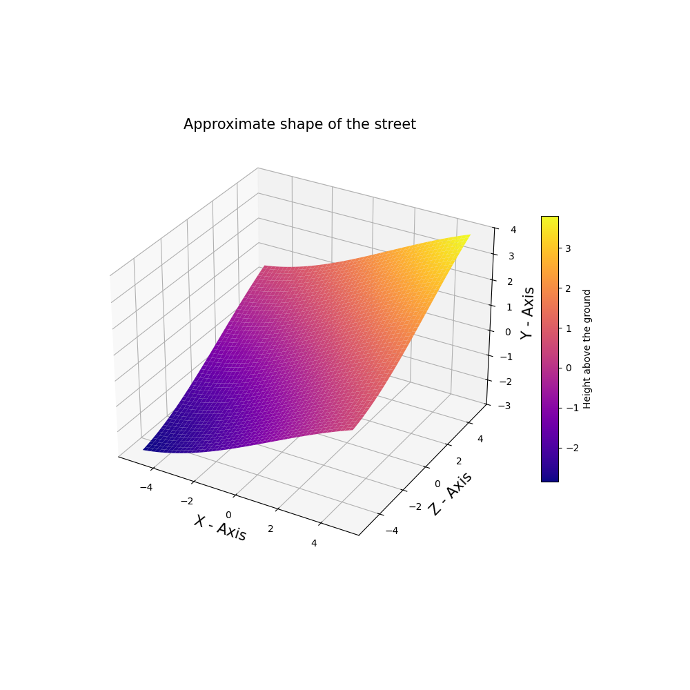
Plot the approximate shape of the street. It does not show the ‘unevenness’.

xs = np.linspace(-lW1, lW1, 500)
ys = np.linspace(-lW1, lW1, 500)
X, Y = np.meshgrid(xs, ys)
Z = gesamt_lam(X, Y, amplitude1, frequenz1)

fig = plt.figure(figsize=(10, 10))
ax = fig.add_subplot(projection='3d')

strasse = ax.plot_surface(X, Y, Z, cmap='plasma', linewidth=0.,
                          antialiased=True)
ax.set_xlabel('X - Axis', fontsize=15)
ax.set_ylabel('Z - Axis', fontsize=15)
ax.set_title('Approximate shape of the street', fontsize=15)
ax.set_zlabel('Y - Axis', fontsize=15)
_ = fig.colorbar(strasse, shrink=0.5, label='Height above the ground',
                 aspect=15)

Animation

This shows the path of the ball, projected on the X / Z plane. The ‘height’ of the ball is indicated by its color.

times2 = []
resultat2 = []

zeitpunkte = 500

reduction = max(1, int(len(times)/zeitpunkte))

for i in range(len(times)):
    if i % reduction == 0:
        times2.append(times[i])
        resultat2.append(resultat[i])

schritte2 = len(times2)
resultat2 = np.array(resultat2)
times2 = np.array(times2)
print('number of points considered:', len(times2))


Dmc1x = np.empty(schritte2)
Dmc1y = np.empty(schritte2)
Dmc1y1 = np.empty(schritte2)
Dmc1z = np.ones(schritte2)

Po1x = np.empty(schritte2)
Po1y = np.empty(schritte2)
Po1z = np.empty(schritte2)

Dmc2x = np.empty(schritte2)
Dmc2y = np.empty(schritte2)
Dmc2y1 = np.empty(schritte2)
Dmc2z = np.ones(schritte2)

Po2x = np.empty(schritte2)
Po2y = np.empty(schritte2)
Po2z = np.empty(schritte2)

for l in range(schritte2):
    Dmc1x[l] = Dmc1_pos_lam(*[resultat2[l, j]
                              for j in range(resultat2.shape[1])], *pL_vals)[0]
    Dmc1y[l] = Dmc1_pos_lam(*[resultat2[l, j]
                              for j in range(resultat2.shape[1])], *pL_vals)[1]
    Dmc1z[l] = Dmc1_pos_lam(*[resultat2[l, j]
                              for j in range(resultat2.shape[1])], *pL_vals)[2]

    Po1x[l] = m_Dmc1_pos_lam(*[resultat2[l, j] for j in
                               range(resultat2.shape[1])], *pL_vals)[0]
    Po1y[l] = m_Dmc1_pos_lam(*[resultat2[l, j] for j in
                             range(resultat2.shape[1])], *pL_vals)[1]
    Po1z[l] = m_Dmc1_pos_lam(*[resultat2[l, j] for j in
                             range(resultat2.shape[1])], *pL_vals)[2]

    Dmc2x[l] = Dmc2_pos_lam(*[resultat2[l, j] for j in
                              range(resultat2.shape[1])], *pL_vals)[0]
    Dmc2y[l] = Dmc2_pos_lam(*[resultat2[l, j] for j in
                              range(resultat2.shape[1])], *pL_vals)[1]
    Dmc2z[l] = Dmc2_pos_lam(*[resultat2[l, j] for j in
                              range(resultat2.shape[1])], *pL_vals)[2]

    Po2x[l] = m_Dmc2_pos_lam(*[resultat2[l, j] for j in
                               range(resultat2.shape[1])], *pL_vals)[0]
    Po2y[l] = m_Dmc2_pos_lam(*[resultat2[l, j] for j in
                               range(resultat2.shape[1])], *pL_vals)[1]
    Po2z[l] = m_Dmc2_pos_lam(*[resultat2[l, j] for j in
                               range(resultat2.shape[1])], *pL_vals)[2]

for i, j in enumerate(Dmc1y):
    Dmc1y1[i] = int(j * 100.)
for i, j in enumerate(Dmc2y):
    Dmc2y1[i] = int(j * 100.)

ymin = min(min(Dmc1y1), min(Dmc2y1))
ymax = max(max(Dmc1y1), max(Dmc2y1))

# This is to asign colors of 'plasma' to the points.
Test = mp.colors.Normalize(ymin, ymax)
Farbe = mp.cm.ScalarMappable(Test, cmap='plasma')
farbe1 = Farbe.to_rgba(Dmc1y1[0])    # color of the starting position
farbe2 = Farbe.to_rgba(Dmc2y1[0])


def animate_pendulum(times, x1, y1, z1, y11, ox, oy, oz, x21, y21, z21, y211,
                     ox1, oy1, oz1):

    fig, ax = plt.subplots(figsize=(8, 8), subplot_kw={'aspect': 'equal'})
    fig.colorbar(Farbe, label=('Height of the ball above ground level'
                               '\n Factor = 100, the real height are the '
                               'numbers divided by factor'), shrink=0.9, ax=ax)
    ax.axis('on')

    ax.set_xlabel(' X Axis', fontsize=18)
    ax.set_ylabel('Z Axis', fontsize=18)

    ax.set(xlim=(-lW1 - 0.9, lW1 + 1.), ylim=(-lW1 - 1., lW1 + 1.))
    ax.plot([-lW1, lW1], [-lW1, -lW1], 'bo', linewidth=2, linestyle='-',
            markersize=0)
    ax.text(0., -lW1-0.5, 'wall 0')
    ax.plot([lW1, lW1], [-lW1, lW1], 'ro', linewidth=2, linestyle='-',
            markersize=0)
    ax.text(lW1 + 0.5, 0., 'wall 1', rotation=90)
    ax.plot([lW1, -lW1], [lW1, lW1], 'go', linewidth=2, linestyle='-',
            markersize=0)
    ax.text(0., lW1 + .5, 'wall 2')
    ax.plot([-lW1, -lW1], [lW1, -lW1], 'yo', linewidth=2, linestyle='-',
            markersize=0)
    ax.text(-lW1-0.5, 0., 'wall 3', rotation=90)

    # Starting point of Dmc1 and Dmc2
    line1,  = ax.plot([], [], 'o', markersize=8, color=farbe1)
    line1a, = ax.plot([], [], 'o', markersize=8, color=farbe2)
    # Moving ball1 and ball2
    line2, = ax.plot([], [], 'o', markersize=90/2.77 * r1 / lW1 * 10.)
    line2a, = ax.plot([], [], 'o', markersize=90/2.77 * r1 / lW1 * 10.)
    # to trace the movement of Dmc1 and Dmc2
    line3,  = ax.plot([], [], color='blue', linewidth=0.25)
    line3a, = ax.plot([], [], color='red', linewidth=0.25)
    # observer on ball 1 and ball 2
    line4,  = ax.plot([], [], 'o', markersize=5, color='black')
    line4a, = ax.plot([], [], 'o', markersize=5, color='black')

    def animate(i):
        farbe3 = Farbe.to_rgba(y11[i])   # color of the actual point at time i
        farbe4 = Farbe.to_rgba(y211[i])  # color of the actual point at time i

        ax.set_title(f'running time {times[i]:.1f} sec, with '
                     f'rumpel = {rumpel}', fontsize=15)

        line1.set_data([x1[0]], [z1[0]])
        line1.set_color(farbe1)
        line1a.set_data([x21[0]], [z21[0]])
        line1a.set_color(farbe2)

        line2.set_data([x1[i]], [z1[i]])
        line2.set_color(farbe3)
        line2a.set_data([x21[i]], [z21[i]])
        line2a.set_color(farbe4)

        line3.set_data(x1[: i], z1[: i])
        line3a.set_data(x21[: i], z21[: i])

        line4.set_data([ox[i]], [oz[i]])
        if y11[i] <= oy[i]:
            line4.set_color('black')
        else:
            line4.set_color('grey')

        line4a.set_data([ox1[i]], [oz1[i]])
        if y211[i] <= oy1[i]:
            line4a.set_color('black')
        else:
            line4a.set_color('grey')

        return line1, line1a, line2, line2a, line3, line3a, line4, line4a

    anim = animation.FuncAnimation(fig, animate, frames=len(times2),
                                   interval=1000*max(times2) / len(times2),
                                   blit=True)
    return anim


anim = animate_pendulum(times2, Dmc1x, Dmc1y, Dmc1z, Dmc1y1, Po1x, Po1y, Po1z,
                        Dmc2x, Dmc2y, Dmc2z, Dmc2y1, Po2x, Po2y, Po2z)


plt.show()

Once Loop Reflect

number of points considered: 536