Linear Tangent Steering (betts_10_73_74)

These are examples 10.73 and 10.74 from John T. Betts, Practical Methods for Optimal Control Using NonlinearProgramming, 3rd edition, Chapter 10: Test Problems. They describe the same problem, but are formulated differently. More details in section 5.6. of the book.

Note

• Both formulations seem to give similar accuracy, but the ‘more complicated’ formulation in example 10.73 solves much faster.

import numpy as np
import sympy as sm
import sympy.physics.mechanics as me
import time
from opty import Problem
from opty.utils import MathJaxRepr
import matplotlib.pyplot as plt

=

Example 10.74

States

• \(x_0, x_1, x_2, x_3\) : state variables

Controls

• \(u\) : control variable

# Equations of motion.

t = me.dynamicsymbols._t

x = me.dynamicsymbols('x:4')
u = me.dynamicsymbols('u')
h = sm.symbols('h')

# Parameter
a = 100.0

eom = sm.Matrix([
    -x[0].diff(t) + x[2],
    -x[1].diff(t) + x[3],
    -x[2].diff(t) + a * sm.cos(u),
    -x[3].diff(t) + a * sm.sin(u),
])
MathJaxRepr(eom)

$$\left[\begin{matrix}x_{2} - \dot{x}_{0}\\x_{3} - \dot{x}_{1}\\100.0 \cos{\left(u \right)} - \dot{x}_{2}\\100.0 \sin{\left(u \right)} - \dot{x}_{3}\end{matrix}\right]$$

Define and Solve the Optimization Problem

num_nodes = 301

t0, tf = 0*h, (num_nodes - 1) * h
interval_value = h

state_symbols = x
unkonwn_input_trajectories = (u, )

Specify the objective function and form the gradient.

def obj(free):
    return free[-1]


def obj_grad(free):
    grad = np.zeros_like(free)
    grad[-1] = 1.0
    return grad

Define the instance constraintsand the bounds. Forcing \(h \geq 0\), avoids physically meaningless negative time intervals.

instance_constraints = (
    x[0].func(t0),
    x[1].func(t0),
    x[2].func(t0),
    x[3].func(t0),
    x[1].func(tf) - 5.0,
    x[2].func(tf) - 45.0,
    x[3].func(tf),
)

bounds = {
        h: (0.0, 0.5),
        u: (-np.pi/2, np.pi/2),
}

Create the optimization problem and set any options.

prob = Problem(
    obj,
    obj_grad,
    eom,
    state_symbols,
    num_nodes,
    interval_value,
    instance_constraints=instance_constraints,
    bounds=bounds,
    time_symbol=t
)

prob.add_option('max_iter', 1000)

Give some rough estimates for the trajectories.

initial_guess = np.ones(prob.num_free)

Find the optimal solution.

start = time.time()
solution, info = prob.solve(initial_guess)
print(f"Time taken to solve: {time.time() - start:.2f} seconds")
print(info['status_msg'])
Jstar = 0.554570879
print(f"Objective value achieved: {info['obj_val']*(num_nodes-1):.4f}, ",
      f"as per the book it is {Jstar:.4f}, so the deviation is: ",
      f"{(info['obj_val']*(num_nodes-1) - Jstar)/Jstar * 100:.4e} %")

solution1 = solution

Time taken to solve: 6.84 seconds
b'Algorithm terminated successfully at a locally optimal point, satisfying the convergence tolerances (can be specified by options).'
Objective value achieved: 0.5546,  as per the book it is 0.5546, so the deviation is:  1.2306e-04 %

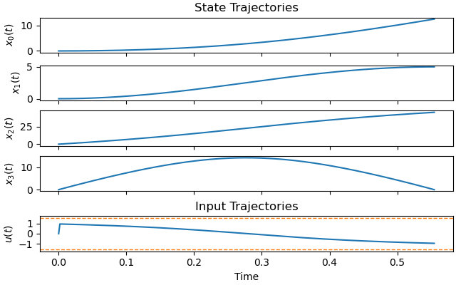
Plot the optimal state and input trajectories.

_ = prob.plot_trajectories(solution, show_bounds=True)

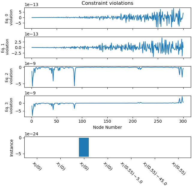
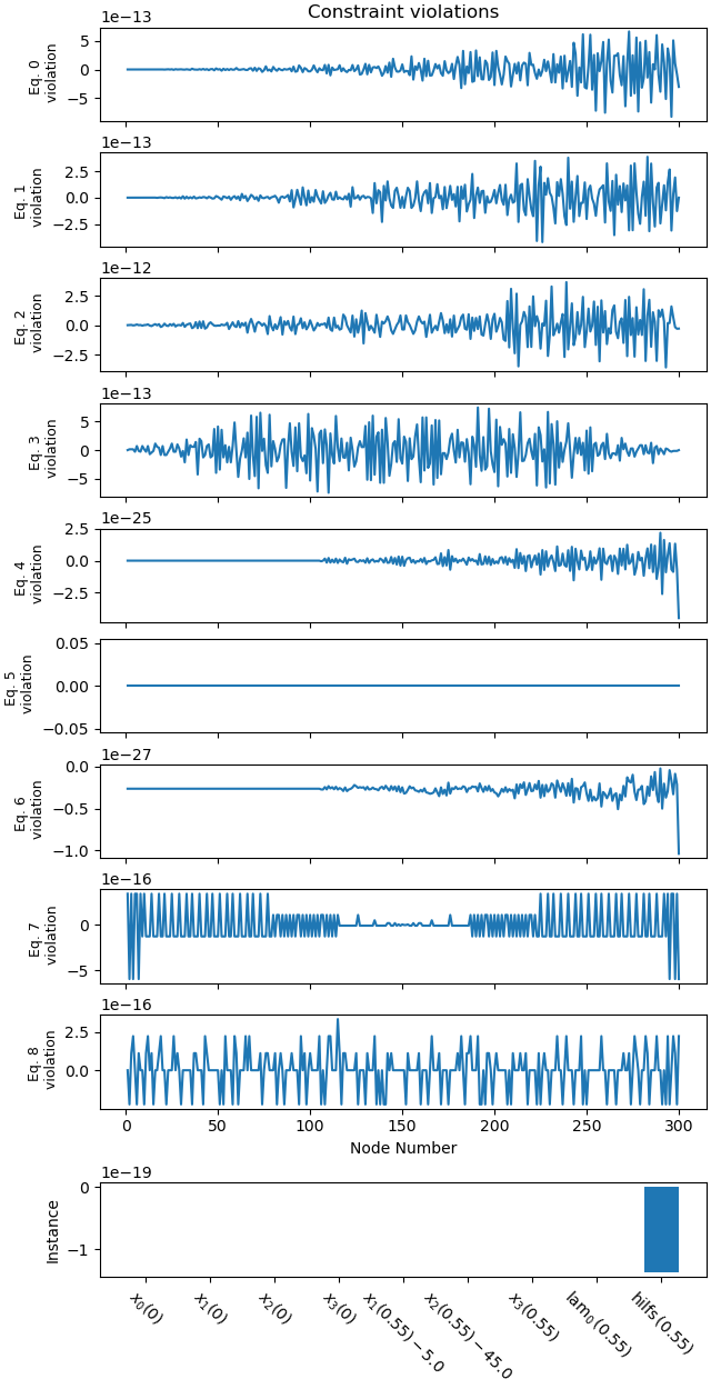
Plot the constraint violations.

_ = prob.plot_constraint_violations(solution, subplots=True)

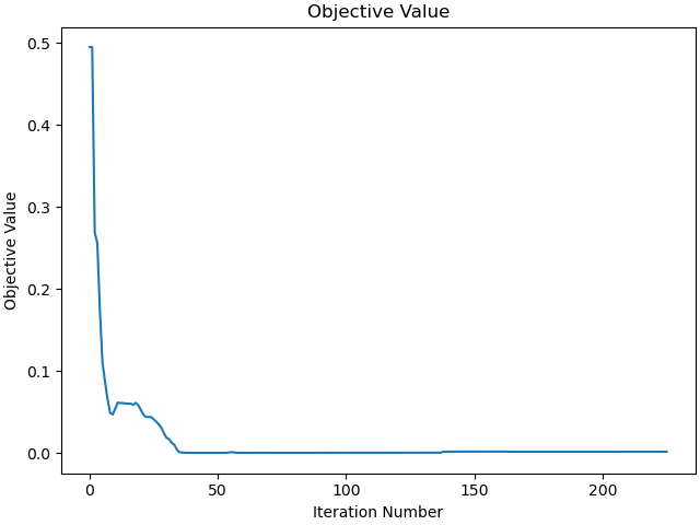
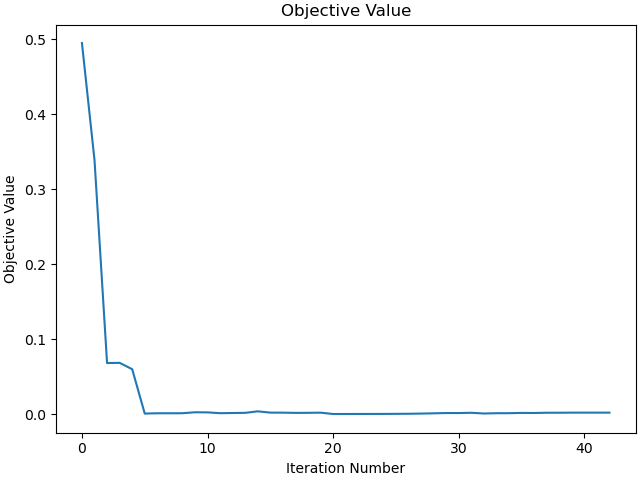
Plot the objective function as a function of optimizer iteration.

_ = prob.plot_objective_value()

Example 10.73

There is a boundary condition at the end of the interval, at \(t = t_f\): \(1 + \lambda_0 x_2 + \lambda_1 x_3 + \lambda_2 a \hspace{2pt} \text{cosu} + \lambda_3 a \hspace{2pt} \text{sinu} = 0\)

where \(\textrm{sinu} = - \lambda_3 / \sqrt{\lambda_2^2 + \lambda_3^2}\) and \(\textrm{cosu} = - \lambda_2 / \sqrt{\lambda_2^2 + \lambda_3^2}\) and a is a constant

As opty presently does not support such instance constraints, I introduce a new state variable and an additional equation of motion:

\(\textrm{hilfs} = 1 + \lambda_0 x_2 + \lambda_1 x_3 + \lambda_2 a \hspace{2pt} \text{cosu} + \lambda_3 a \hspace{2pt} \text{sinu}\)

and the instance constraint \(\textrm{hilfs}(t_f) = 0\) is used.

states

• \(x_0, x_1, x_2, x_3\) : state variables

• \(\textrm{lam}_0, \textrm{lam}_1, \textrm{lam}_2, \textrm{lam}_3\) : state variables

• \(\textrm{hilfs}\) : state variable

Equations of Motion

t = me.dynamicsymbols._t

x = me.dynamicsymbols('x:4')
lam = me.dynamicsymbols('lam:4')
hilfs = me.dynamicsymbols('hilfs')
h = sm.symbols('h')

# Parameters
a = 100.0

cosu = - lam[2] / sm.sqrt(lam[2]**2 + lam[3]**2)
sinu = - lam[3] / sm.sqrt(lam[2]**2 + lam[3]**2)

eom = sm.Matrix([
    -x[0].diff(t) + x[2],
    -x[1].diff(t) + x[3],
    -x[2].diff(t) + a * cosu,
    -x[3].diff(t) + a * sinu,
    -lam[0].diff(t),
    -lam[1].diff(t),
    -lam[2].diff(t) - lam[0],
    -lam[3].diff(t) - lam[1],
    -hilfs + 1 + lam[0]*x[2] + lam[1]*x[3] + lam[2]*a*cosu + lam[3]*a*sinu,
])
MathJaxRepr(eom)

$$\left[\begin{matrix}x_{2} - \dot{x}_{0}\\x_{3} - \dot{x}_{1}\\- \dot{x}_{2} - \frac{100.0 lam_{2}}{\sqrt{lam_{2}^{2} + lam_{3}^{2}}}\\- \dot{x}_{3} - \frac{100.0 lam_{3}}{\sqrt{lam_{2}^{2} + lam_{3}^{2}}}\\- \dot{lam}_{0}\\- \dot{lam}_{1}\\- lam_{0} - \dot{lam}_{2}\\- lam_{1} - \dot{lam}_{3}\\- hilfs + lam_{0} x_{2} + lam_{1} x_{3} + 1 - \frac{100.0 lam_{2}^{2}}{\sqrt{lam_{2}^{2} + lam_{3}^{2}}} - \frac{100.0 lam_{3}^{2}}{\sqrt{lam_{2}^{2} + lam_{3}^{2}}}\end{matrix}\right]$$

Define and Solve the Optimization Problem

state_symbols = x + lam + [hilfs]

t0, tf = 0*h, (num_nodes - 1) * h
interval_value = h

Specify the objective function and form the gradient.

def obj(free):
    return free[-1]


def obj_grad(free):
    grad = np.zeros_like(free)
    grad[-1] = 1.0
    return grad


instance_constraints = (
    x[0].func(t0),
    x[1].func(t0),
    x[2].func(t0),
    x[3].func(t0),
    x[1].func(tf) - 5.0,
    x[2].func(tf) - 45.0,
    x[3].func(tf),
    lam[0].func(tf),
    hilfs.func(tf),
)

bounds = {
        h: (0.0, 0.5),
}

Create the optimization problem and set any options.

prob = Problem(
    obj,
    obj_grad,
    eom,
    state_symbols,
    num_nodes,
    interval_value,
    instance_constraints=instance_constraints,
    bounds=bounds,
    time_symbol=t
)

prob.add_option('max_iter', 1000)

Give some rough estimates for the trajectories.

initial_guess = np.ones(prob.num_free)

Find the optimal solution.

start = time.time()
solution, info = prob.solve(initial_guess)
print(f"Time taken to solve: {time.time() - start:.2f} seconds")
print(info['status_msg'])
Jstar = 0.554570879
print(f"Objective value achieved: {info['obj_val']*(num_nodes-1):.4f}, ",
      f"as per the book it is {Jstar:.4f}, so the deviation is: ",
      f"{(info['obj_val']*(num_nodes-1) - Jstar)/Jstar * 100:.4e} %")

Time taken to solve: 1.61 seconds
b'Algorithm terminated successfully at a locally optimal point, satisfying the convergence tolerances (can be specified by options).'
Objective value achieved: 0.5546,  as per the book it is 0.5546, so the deviation is:  1.2300e-04 %

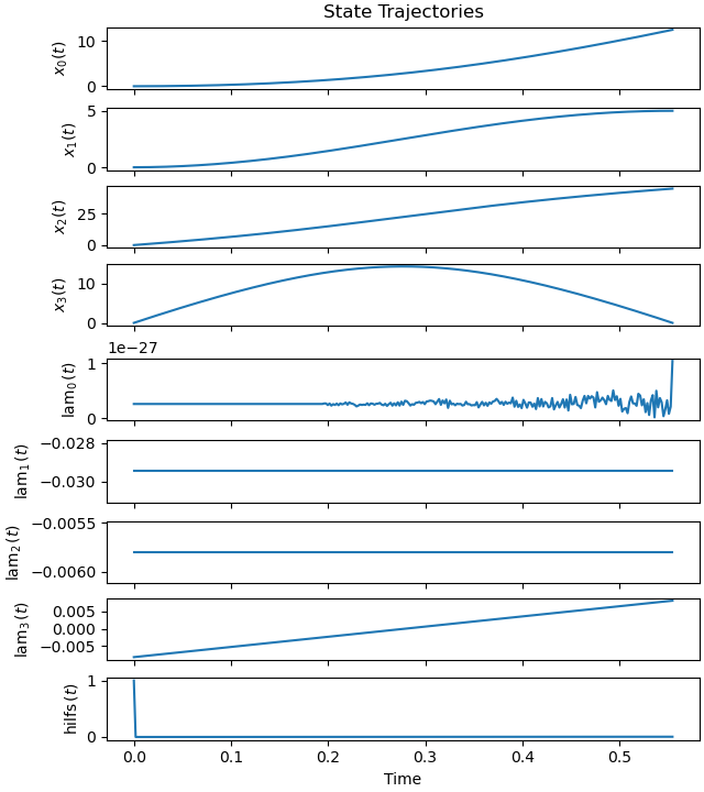
Plot the optimal state and input trajectories.

_ = prob.plot_trajectories(solution)

Plot the constraint violations.

_ = prob.plot_constraint_violations(solution, subplots=True)

Plot the objective function as a function of optimizer iteration.

_ = prob.plot_objective_value()

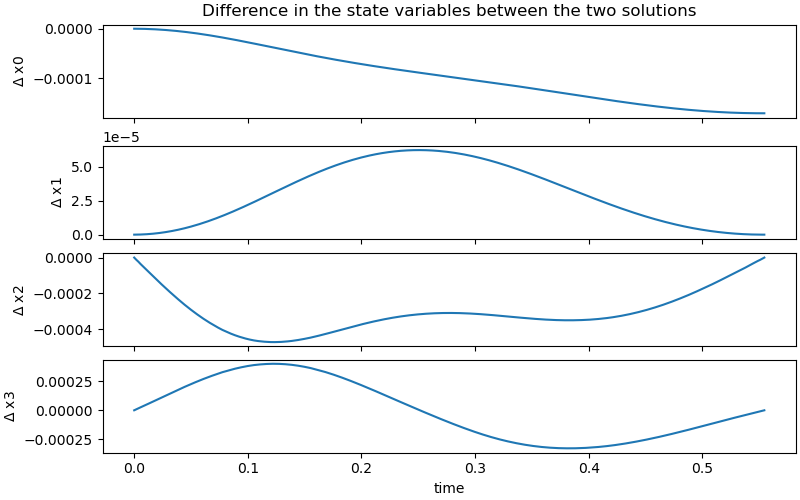
Compare the two solutions.

difference = np.empty(4*num_nodes)
for i in range(4*num_nodes):
    difference[i] = solution1[i] - solution[i]

fig, ax = plt.subplots(4, 1, figsize=(8, 5), layout='constrained', sharex=True)
names = ['x0', 'x1', 'x2', 'x3']
times = np.linspace(t0, (num_nodes-1)*solution[-1], num_nodes)
msg = r"$\Delta$"
for i in range(4):
    ax[i].plot(times, difference[i*num_nodes:(i+1)*num_nodes])
    ax[i].set_ylabel(f'{msg} {names[i]}')
ax[0].set_title('Difference in the state variables between the two solutions')
_ = ax[-1].set_xlabel('time')