Rolling Axle on Flat Surface

Objectives

• If rolling without slipping is assumed, the contact points have zero velocity. Show how to use this to get the dependent speeds with a simple example.

• The nonlinear holonomic constraints seem to have several solutions, not all of them meet physical reality. Solving them with random initial guesses and checking whether physical reality is met seems a doable approach.

Description

Two wheels of radii \(r_L\) and \(r_R\) and masses \(m_L\) and \(m_R\) are connected by an axle of length \(l\). They can rotate independently around the axle. This ‘system’ rolls on a horizontal plane without slipping. A particle of mass \(m_p\) is attached to each wheel.

States

• \(x_L\) : the X coordinate of the left contact point

• \(y_L\) : the Y coordinate of the left contact point

• \(x_R\) : the X coordinate of the right contact point

• \(y_R\) : the Y coordinate of the right contact point

• \(q_2\) : the angle between the axle and the horizontal plane. This is given by the geometry of the system and does not change during the motion. it is not a state variable.

• \(q_3\) : the rotation of the axle in the plane

• \(q_L\) : the rotation of the left wheel around the axle

• \(q_R\) : the rotation of the right wheel around the axle

• \(u_L\) : the speed of \(q_L\)

• \(u_R\) : the speed of \(q_R\)

• \(u_3\) : the speed of \(q_3\)

Parameters

• \(g\) : gravitational acceleration

• \(m_L\) : mass of the left wheel

• \(m_R\) : mass of the right wheel

• \(m_p\) : mass of the particles attached to the wheels

• \(r_L\) : radius of the left wheel

• \(r_R\) : radius of the right wheel

• \(l\) : length of the axle

import sympy as sm
import sympy.physics.mechanics as me
import numpy as np
import matplotlib.pyplot as plt

from scipy.optimize import root
from scipy.integrate import solve_ivp
from scipy.interpolate import interp1d
from opty.utils import MathJaxRepr
from matplotlib.animation import FuncAnimation
from matplotlib.patches import Ellipse
from matplotlib.transforms import Affine2D

Set the frames and the points.

N, AX, AL, AR = sm.symbols('N AX AL AR', cls=me.ReferenceFrame)
O, DmcL, DmcR, CPL, CPR = sm.symbols('O DmcL DmcR CPL CPR',
                                     cls=me.Point)
p_L, p_R = sm.symbols('p_L p_R', cls=me.Point)
t = me.dynamicsymbols._t
O.set_vel(N, 0)

Location of the contact points in N.

xL, yL, zL, xR, yR, zR = me.dynamicsymbols('xL yL zL xR yR zR')
uxL, uyL, uzL, uxR, uyR, uzR = me.dynamicsymbols('uxL uyL uzL uxR uyR uzR')

Components of the vector from CPL to DmcL in AX.

lx, ly, lz = sm.symbols('lx ly lz')

Rotations of the wheels in AL, AR respectively.

qL, qR, uqL, uqR = me.dynamicsymbols('qL qR uqL uqR')

Rotation of the axle in N. It does not rotatate around itself. Masses, radii and inertia of the wheels. length of the axle is l

g, mL, mR, mp, rL, rR, l = sm.symbols('g mL mR mp rL rR l')

q3, u3 = me.dynamicsymbols('q3 u3')
winkel_q2 = sm.atan((rL - rR) / l)
AX.orient_body_fixed(N, [q3, winkel_q2, 0], 'ZYX')

Rotation of the wheels.

AL.orient_axis(AX, qL, AX.x)
AR.orient_axis(AX, qR, AX.x)

Position of the contact points.

CPL.set_pos(O, xL * N.x + yL * N.y)
CPR.set_pos(O, xR * N.x + yR * N.y)

Attach the particle.

p_L.set_pos(DmcL, rL/2*AL.y)
p_R.set_pos(DmcR, -rR/2*AR.y)

Define a dictionary needed later.

kin_dict = {
    xL.diff(t): uxL,
    yL.diff(t): uyL,
    xR.diff(t): uxR,
    yR.diff(t): uyR,
    qL.diff(t): uqL,
    qR.diff(t): uqR,
    q3.diff(t): u3,
}

Define the vectors from the contact points to the center of the wheels. Note that \(\text{vector}_L \parallel \text{vector}_R\) at all times, but different lengths.

stretch = rR/rL
vectorL = lx*AX.x + ly*AX.y + lz*AX.z
vectorR = stretch * vectorL

DmcR can be defined two ways. This is used to get constraints. DmcR_h is physically the same point as DmcR.

DmcR_h = me.Point('DmcR_h')

DmcL.set_pos(CPL, vectorL)
DmcR.set_pos(CPR, vectorR)
DmcR_h.set_pos(DmcL, l*AX.x)

Holonomic constraints.

Conditions \(l_x, l_y, l_z\) must meet.

constr_liri = sm.Matrix([
    vectorL.dot(AX.x),  # left wheel perpendicular to the axle
    vectorL.dot(AX.y),  # left wheel perpendicular to the AX.y
    vectorL.magnitude() - rL,   # left wheel radius
])

Additional constraint: DmcR and DmcR_h are at the same position at all times. Five constraints are needed to get \(l_x, l_y, l_z\) and the initial position of \(x_R, y_R\) given \(q_3\)

constr_DmcR = sm.Matrix([
    (DmcR.pos_from(O) - DmcR_h.pos_from(O)).dot(N.x),
    (DmcR.pos_from(O) - DmcR_h.pos_from(O)).dot(N.y),
])

constr_all = constr_liri.col_join(constr_DmcR)
print('constr_all DS', me.find_dynamicsymbols(constr_all))
print('constr_all free symbols', constr_all.free_symbols)
MathJaxRepr(constr_all)

constr_all DS {xR(t), yL(t), yR(t), xL(t), q3(t)}
constr_all free symbols {rL, rR, l, lz, lx, ly, t}

$$\left[\begin{matrix}lx\\ly\\- rL + \sqrt{lx^{2} + ly^{2} + lz^{2}}\\- \left(- ly + \frac{ly rR}{rL}\right) \sin{\left(q_{3} \right)} - xL + xR + \frac{\left(- l - lx + \frac{lx rR}{rL}\right) \cos{\left(q_{3} \right)}}{\sqrt{1 + \frac{\left(rL - rR\right)^{2}}{l^{2}}}} + \frac{\left(- lz + \frac{lz rR}{rL}\right) \left(rL - rR\right) \cos{\left(q_{3} \right)}}{l \sqrt{1 + \frac{\left(rL - rR\right)^{2}}{l^{2}}}}\\\left(- ly + \frac{ly rR}{rL}\right) \cos{\left(q_{3} \right)} - yL + yR + \frac{\left(- l - lx + \frac{lx rR}{rL}\right) \sin{\left(q_{3} \right)}}{\sqrt{1 + \frac{\left(rL - rR\right)^{2}}{l^{2}}}} + \frac{\left(- lz + \frac{lz rR}{rL}\right) \left(rL - rR\right) \sin{\left(q_{3} \right)}}{l \sqrt{1 + \frac{\left(rL - rR\right)^{2}}{l^{2}}}}\end{matrix}\right]$$

Nonholonomic Constraints

CPL and CPR have zero speed as we assume rolling. Dependent speeds are: \(ux_L, uy_L, ux_R, uy_R, u3\)

DmcL.set_vel(N, DmcL.pos_from(O).diff(t, N))
DmcR.set_vel(N, DmcR.pos_from(O).diff(t, N))
vDmcL = DmcL.vel(N).subs(kin_dict)
vDmcR = DmcR.vel(N).subs(kin_dict)

CPL.set_vel(N, vDmcL + AL.ang_vel_in(N).cross(-vectorL))
CPR.set_vel(N, vDmcR + AR.ang_vel_in(N).cross(-vectorR))
vCPL = CPL.vel(N).subs(kin_dict)
vCPR = CPR.vel(N).subs(kin_dict)

No slip condition. CPL, CPR must have zero speed in N. As five conditions are needed to get the five dependent speeds, the time derivative of the last holonomic constraint is added to the list of the speed constraints. Maybe a bit arbitrary.

constr_noslip = sm.Matrix([
    vCPL.dot(N.x),
    vCPL.dot(N.y),
    vCPR.dot(N.x),
    vCPR.dot(N.y),
    constr_all[-1].diff(t),
]).subs(kin_dict)

Solve the speed constraints for the dependent speeds.

Mk = constr_noslip.jacobian(sm.Matrix([uxL, uyL, uxR, uyR, u3]))
gk = constr_noslip.subs({uxL: 0, uyL: 0, uxR: 0, uyR: 0, u3: 0})
loesung = Mk.LUsolve(-gk)
print('loesung dynamic symbols =', me.find_dynamicsymbols(loesung))

loesung dynamic symbols = {uqR(t), uqL(t), q3(t)}

Kane’s equations

iXXL = 0.5 * mL * rL**2
iYYL = 0.25 * mL * rL**2
iZZL = iYYL
iXXR = 0.5 * mR * rR**2
iYYR = 0.25 * mR * rR**2
iZZR = iYYR
inertiaL = me.inertia(AL, iXXL, iYYL, iZZL)
inertiaR = me.inertia(AR, iXXR, iYYR, iZZR)
wheelL = me.RigidBody('wheelL', DmcL, AL, mL, (inertiaL, DmcL))
wheelR = me.RigidBody('wheelR', DmcR, AR, mR, (inertiaR, DmcR))
partL = me.Particle('partL', p_L, mp)
partR = me.Particle('partR', p_R, mp)
bodies = [wheelL, wheelR, partL, partR]

forces = [(DmcL, -mL * g * N.z), (DmcR, -mR * g * N.z),
          (p_L, -mp * g * N.z), (p_R, -mp * g * N.z)]

speed_constr = [
    uxL - loesung[0],
    uyL - loesung[1],
    uxR - loesung[2],
    uyR - loesung[3],
    u3 - loesung[4],
]

kd = sm.Matrix([
    xL.diff(t) - uxL,
    yL.diff(t) - uyL,
    xR.diff(t) - uxR,
    yR.diff(t) - uyR,
    q3.diff(t) - u3,
    qR.diff(t) - uqR,
    qL.diff(t) - uqL,
])

q_ind = [xL, yL, xR, yR, q3, qR, qL]
u_ind = [uqL, uqR]
u_dep = [uxL, uyL, uxR, uyR, u3]

kane = me.KanesMethod(
    N,
    q_ind,
    u_ind,
    u_dependent=u_dep,
    kd_eqs=kd,
    velocity_constraints=speed_constr,
)

fr, frstar = kane.kanes_equations(bodies, forces)

MM = kane.mass_matrix_full
force = kane.forcing_full

print(f"force contains {sm.count_ops(force)} operations")
print("force free symbols =", force.free_symbols)
print("force dynamic symbols =", me.find_dynamicsymbols(force), '\n')
print(f"MM contains {sm.count_ops(MM)} operations")
print("MM free symbols =", MM.free_symbols)
print("MM dynamic symbols =", me.find_dynamicsymbols(MM), '\n')

force contains 21768 operations
force free symbols = {mR, rL, mL, rR, l, lz, ly, mp, t, lx, g}
force dynamic symbols = {uxR(t), qR(t), uyL(t), uqR(t), q3(t), uyR(t), u3(t), uxL(t), uqL(t), qL(t)}

MM contains 20243 operations
MM free symbols = {mR, rL, mL, rR, l, lz, ly, mp, t, lx}
MM dynamic symbols = {qR(t), q3(t), qL(t)}

Energies.

kin_energy = sum([body.kinetic_energy(N).subs(kin_dict) for body in bodies])
pot__energy = sum([g * body.mass * body.masscenter.pos_from(O).dot(N.z)
                   for body in bodies])

Compilation.

qL = q_ind + u_ind + u_dep
pL = [lx, ly, lz, g, mL, mR, mp, rL, rR, l]

MM_lam = sm.lambdify(qL + pL, MM, cse=True)
force_lam = sm.lambdify(qL + pL, force, cse=True)

constr_all_lam = sm.lambdify([xR, yR, lx, ly, lz] +
                             [xL, yL, q3] +
                             pL[3:], constr_all, cse=True)

loesung_lam = sm.lambdify([uqL, uqR, q3] + pL, loesung, cse=True)


vecLdotAXx = vectorL.dot(AX.x)
vecLdotAXy = vectorL.dot(AX.y)
dot_lam = sm.lambdify([lx, ly, lz, rL, rR, l, q3],
                      [vecLdotAXx, vecLdotAXy], cse=True)

vCPL_lam = sm.lambdify(qL + pL, [vCPL.dot(N.x), vCPL.dot(N.y),
                                 vCPL.dot(N.z)], cse=True)
vCPR_lam = sm.lambdify(qL + pL, [vCPR.dot(N.x), vCPR.dot(N.y),
                                 vCPR.dot(N.z)], cse=True)

vDmcL_lam = sm.lambdify(qL + pL, [DmcL.vel(N).subs(kin_dict).dot(N.x),
                                  DmcL.vel(N).subs(kin_dict).dot(N.y),
                                  DmcL.vel(N).subs(kin_dict).dot(N.z)],
                        cse=True)
vDmcR_lam = sm.lambdify(qL + pL, [DmcR.vel(N).subs(kin_dict).dot(N.x),
                                  DmcR.vel(N).subs(kin_dict).dot(N.y),
                                  DmcR.vel(N).subs(kin_dict).dot(N.z)],
                        cse=True)

kin_lam = sm.lambdify(qL + pL, kin_energy, cse=True)
pot_lam = sm.lambdify(qL + pL, pot__energy, cse=True)

Just for easy plotting.

constr_all_plot_lam = sm.lambdify(qL + pL, constr_all, cse=True)
CPRfromCPL_lam = sm.lambdify(qL + pL, CPR.pos_from(CPL).
                             magnitude().subs(kin_dict), cse=True)
DmcRfromDmcL_lam = sm.lambdify(qL + pL, DmcR.pos_from(DmcL).
                               magnitude().subs(kin_dict), cse=True)
DmcLfromO_lam = sm.lambdify(qL + pL, [DmcL.pos_from(O).dot(N.x).subs(kin_dict),
                                      DmcL.pos_from(O).dot(N.y).subs(kin_dict),
                                      DmcL.pos_from(O).dot(N.z).
                                      subs(kin_dict)], cse=True)
DmcRfromO_lam = sm.lambdify(qL + pL, [DmcR.pos_from(O).dot(N.x).subs(kin_dict),
                                      DmcR.pos_from(O).dot(N.y).subs(kin_dict),
                                      DmcR.pos_from(O).dot(N.z).
                                      subs(kin_dict)], cse=True)

Set initial values, calculate dependent initial conditions.

mL1 = 1.0
mR1 = 1.0
mp1 = 1.0
rL1 = 1.0
rR1 = 2.0
l1 = 2.0
g1 = 9.81

xL1 = 10.0
yL1 = 0.0
qL1 = 0.0
qR1 = 0.0
q31 = 0.0

uqL1 = -1.0
uqR1 = 1.0


def func_all(x0, args):
    xR1, yR1, lx1, ly1, lz1 = x0
    xL1, yL1, q31, g1, mL1, mR1, mp1, rL1, rR1, l1 = args
    return constr_all_lam(xR1, yR1, lx1, ly1, lz1,
                          xL1, yL1, q31, g1, mL1, mR1, mp1, rL1, rR1,
                          l1).squeeze()


args = [xL1, yL1, q31, g1, mL1, mR1, mp1, rL1, rR1, l1]

Solve the nonlinear holonomic constraints for the initial conditions. There seem to be several solution, which do not meet the physical reality. So I iterate over random initial guesses until I get a solution that meets the physical reality.

np.random.seed(12)
for i in range(500):
    try:
        x0 = np.random.uniform(-4, 4, 5)
        res = root(func_all, x0, args=args)
        if (res.success
            and np.allclose(np.sqrt(res.x[2]**2 + res.x[3]**2 + res.x[4]**2),
                            rL1, atol=1e-9)
            and np.sqrt((xL1 - res.x[0])**2 + (yL1 - res.x[1])**2) >= l1
            and res.x[4] > 0):
            break
    except Exception as e:
        print(f"Attempt {i+1} failed: {e}")

print('loops needed', i + 1)
print(res.message)
xR1, yR1, lx1, ly1, lz1 = res.x
radiusL = np.sqrt(lx1**2 + ly1**2 + lz1**2)
print('radiusL =', radiusL)
print('CPR distance from CPL =',
      anfangs_dist := np.sqrt((xL1 - res.x[0])**2 + (yL1 - res.x[1])**2))
print(f'scalar prodct between vectorl and AX.x is '
      f'{dot_lam(lx1, ly1, lz1, rL1, rR1, l1, q31)[0]:.2e}',
      f'between vectorL and AX.y it is '
      f'{dot_lam(lx1, ly1, lz1, rL1, rR1, l1, q31)[1]:.2e}')
print(f"angle q2: {np.rad2deg(np.tan((rL1 - rR1) / l1)):.1f} deg")

loops needed 6
The solution converged.
radiusL = 0.9999999999999999
CPR distance from CPL = 2.23606797749979
scalar prodct between vectorl and AX.x is -8.30e-25 between vectorL and AX.y it is -2.55e-24
angle q2: -31.3 deg

Calculate dependent speeds, using the results obtained above.

dep_vel = loesung_lam(uqL1, uqR1, q31, lx1, ly1, lz1, g1, mL1, mR1, mp1,
                      rL1, rR1, l1)
# uxL, uyL, uxR, uyR, u3
uxL1 = dep_vel[0][0]
uyL1 = dep_vel[1][0]
uxR1 = dep_vel[2][0]
uyR1 = dep_vel[3][0]
u3 = dep_vel[4][0]

Get the sequence of the many variables right in \(y_0, pL_{vals}\)

q_ind = [xL, yL, xR, yR, q3, qR, qL]

u_ind = [uqL, uqR]

u_dep = [uxL, uyL, uxR, uyR, u3]

y0 = [xL1, yL1, xR1, yR1, q31, qR1, qL1, uqL1, uqR1, uxL1, uyL1, uxR1, uyR1,
      u3]

# pL = [lx, ly, lz, g, mL, mR, mp, rL, rR, l]
pL_vals = [lx1, ly1, lz1, g1, mL1, mR1, mp1, rL1, rR1, l1]

print(f"norm of speed of CPL is {np.linalg.norm(vCPL_lam(*y0, *pL_vals)):.3e}")
print(f"norm of speed of CPR is {np.linalg.norm(vCPR_lam(*y0, *pL_vals)):.3e}")

norm of speed of CPL is 2.220e-16
norm of speed of CPR is 1.110e-16

Numerical Integration

intervall = 10.0
punkte = 100
schritte = int(intervall * punkte)

times = np.linspace(0, intervall, schritte)


def gradient(t, y, args):
    sol = np.linalg.solve(MM_lam(*y, *args), force_lam(*y, *args))
    return np.array(sol).T[0]


t_span = (0., intervall)
resultat1 = solve_ivp(gradient, t_span, y0, t_eval=times, args=(pL_vals,),
                      atol=1.e-9,
                      rtol=1.e-9,
                      )

resultat = resultat1.y.T
print(resultat.shape)
print(resultat1.message, resultat1.t[-1])

print('resultat shape', resultat.shape, '\n')

print(f"To numerically integrate an intervall of {intervall} sec, "
      f"the routine cycled {resultat1.nfev} times")

(1000, 14)
The solver successfully reached the end of the integration interval. 10.0
resultat shape (1000, 14)

To numerically integrate an intervall of 10.0 sec, the routine cycled 1430 times

Plot some generalized coordinates / speeds, etc.

bezeichnung = [str(i) for i in qL]
fig, ax = plt.subplots(7, 1, figsize=(10, 12), sharex=True,
                       layout='constrained')
for i in (0, 1, 2, 3, 4):
    ax[0].plot(times, resultat[:, i], label=bezeichnung[i])
ax[-1].set_xlabel('time (s)')
ax[0].set_title(f"Generalized coordinates, radius of left wheel = {rL1}, "
                f"radius of right wheel = {rR1}")
_ = ax[0].legend()

vCPL_np = np.array([vCPL_lam(*row, *pL_vals) for row in resultat])
vCPR_np = np.array([vCPR_lam(*row, *pL_vals) for row in resultat])
ax[1].plot(times, vCPL_np[:, 0], label='CPL x')
ax[1].plot(times, vCPL_np[:, 1], label='CPL y')
ax[1].plot(times, vCPL_np[:, 2], label='CPL z')
ax[1].plot(times, vCPR_np[:, 0], label='CPR x')
ax[1].plot(times, vCPR_np[:, 1], label='CPR y')
ax[1].plot(times, vCPR_np[:, 2], label='CPR z')
ax[1].set_title('Velocity of contact points')
_ = ax[1].legend()

kin_np = np.array([kin_lam(*row, *pL_vals) for row in resultat])
pot_np = np.array([pot_lam(*row, *pL_vals) for row in resultat])
total_np = kin_np + pot_np
ax[2].plot(times, kin_np, label='kinetic energy')
ax[2].plot(times, pot_np, label='potential energy')
ax[2].plot(times, total_np, label='total energy')
ax[2].set_title('Energies')
_ = ax[2].legend()

max_total = np.max(total_np)
min_total = np.min(total_np)
deviation = (max_total - min_total) / max_total * 100
print("max. deviation of the total energy from being constant is "
      f"{deviation:.2e} %")

vDmcL_np = np.array([vDmcL_lam(*row, *pL_vals) for row in resultat])
vDmcR_np = np.array([vDmcR_lam(*row, *pL_vals) for row in resultat])
ax[3].plot(times, vDmcL_np[:, 0], label='DmcL x')
ax[3].plot(times, vDmcL_np[:, 1], label='DmcL y')
ax[3].plot(times, vDmcL_np[:, 2], label='DmcL z')
ax[3].plot(times, vDmcR_np[:, 0], label='DmcR x')
ax[3].plot(times, vDmcR_np[:, 1], label='DmcR y')
ax[3].plot(times, vDmcR_np[:, 2], label='DmcR z')
ax[3].set_title('Velocity of center points')
ax[3].legend()


namen = [
    r'vectorL $\perp$ AX.x',
    r'vectorL $\perp$ AX.y',
    r'|vectorL| $\approx r_L$',
    r'close to DmcR - DmcR_h in x',
    r'close to DmcR - DmcR_h in y',
]
constr_all_np = np.array([constr_all_plot_lam(*row, *pL_vals)
                          for row in resultat]).squeeze(-1)
for i in range(0, constr_all_np.shape[1]):
    ax[4].plot(times, constr_all_np[:, i], label=namen[i])
ax[4].set_title('Error in the Constraints')
ax[4].legend()

CPRfromCPL_np = np.array([CPRfromCPL_lam(*row, *pL_vals) for row in resultat])
ax[5].plot(times, CPRfromCPL_np, label='Distance from CPL to CPR')
ax[5].axhline(anfangs_dist, color='red', linestyle='--',
              label='correct distance')
ax[5].set_title('Distance from CPL to CPR')
ax[5].legend()

DmcRfromDmcL_np = np.array([DmcRfromDmcL_lam(*row, *pL_vals)
                            for row in resultat])
ax[6].axhline(l1, color='red', linestyle='--', label='correct distance')
ax[6].set_title('Distance from left to right hub')
ax[6].plot(times, DmcRfromDmcL_np)
_ = ax[6].legend()

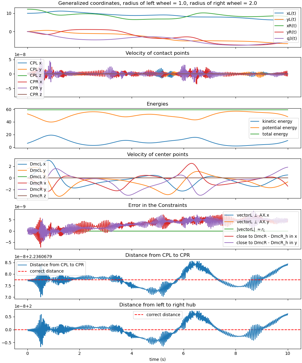
max. deviation of the total energy from being constant is 5.02e-07 %

2D Animation

Looking down on the system from above.

fps = 25

t_arr = times
state_sol = interp1d(t_arr, resultat, kind='cubic', axis=0)

coordinates = DmcL.pos_from(O).to_matrix(N)
for point in (DmcR, p_L, p_R):
    coordinates = coordinates.row_join(point.pos_from(O).to_matrix(N))

coords_lam = sm.lambdify(qL + pL, coordinates, cse=True)

max_x = np.max(np.concatenate((resultat[:, 0], resultat[:, 2])))
max_y = np.max(np.concatenate((resultat[:, 1], resultat[:, 3])))
min_x = np.min(np.concatenate((resultat[:, 0], resultat[:, 2])))
min_y = np.min(np.concatenate((resultat[:, 1], resultat[:, 3])))

fig, ax = plt.subplots(figsize=(7, 7))
ax.set_xlim(min_x-1, max_x+1)
ax.set_ylim(min_y-1, max_y+1)
ax.set_aspect('equal')
ax.set_xlabel('x', fontsize=15)
ax.set_ylabel('y', fontsize=15)

line1, = ax.plot([], [], lw=1, marker='o', markersize=0, color='red')
line4 = ax.scatter([], [], color='black', s=20)
line5 = ax.scatter([], [], color='black', s=20)

# ellipses defined in local frame AX
winkel_q2 = np.atan((rL1 - rR1) / l1)
ellipseL = Ellipse((0, 0), width=rL1*np.sin(winkel_q2), height=rL1,
                   fill=True, lw=2, color='green', alpha=0.5)
ax.add_patch(ellipseL)
EllipseR = Ellipse((0, 0), width=rR1*np.sin(winkel_q2), height=rR1,
                   fill=True, lw=2, color='blue', alpha=0.5)
ax.add_patch(EllipseR)


def update(t):
    message = (f'running time {t:.2f} sec \n'
               f'the left wheel is green with radius {rL1}, the right wheel '
               f'is blue with radius {rR1} \n'
               'The black dots are the particles attached to the wheels')
    ax.set_title(message, fontsize=12)
    coords = coords_lam(*state_sol(t), *pL_vals)

    line1.set_data([coords[0, 0], coords[0, 1]], [coords[1, 0],
                                                  coords[1, 1]])
    line4.set_offsets([coords[0, 2], coords[1, 2]])
    line5.set_offsets([coords[0, 3], coords[1, 3]])

    # transform from AX → inertial frame
    theta = state_sol(t)[4]
    X = coords[0, 0]
    Y = coords[1, 0]
    transform = Affine2D().rotate(theta).translate(X, Y) + ax.transData
    ellipseL.set_transform(transform)
    X = coords[0, 1]
    Y = coords[1, 1]
    transform = Affine2D().rotate(theta).translate(X, Y) + ax.transData
    EllipseR.set_transform(transform)

    return line1, line4, line5, ellipseL, EllipseR


# Create the animation
animation = FuncAnimation(fig, update, frames=np.arange(0, intervall, 1.0/fps),
                          interval=1500/fps, blit=False)
plt.show()

Once Loop Reflect