Rattleback

Objectives

• Show how to define a special ode_solver, needed here for accuracy.

• Show how to use PyDy’s ecaluate_holonomic and evaluate_nonholonomic functions to see how well the constraints are satisfied.

Description

This simulation is taken from this article: https://www.sciencedirect.com/science/article/abs/pii/0020746282900178 The equations of motion are set up using Kane’s method from SymPy’s physics.mechanics module. The ingenious way to get the contact points of the rattleback with the plane is from the paper.

Notes

• The numerical integration seems quite difficult. Even with ‘’method=DOP853’’, which is a high order method, the standard values of atol and rtol are not sufficient to get a qualitatively reasonable result.

• It seems to depend critically on the constants, also taken from the a.m. paper. (Maybe this is the reason rattleback are not seen often in nature)

• While 0.9.4 is the latest released version of PyDy, the development version of PyDy must be used.

States

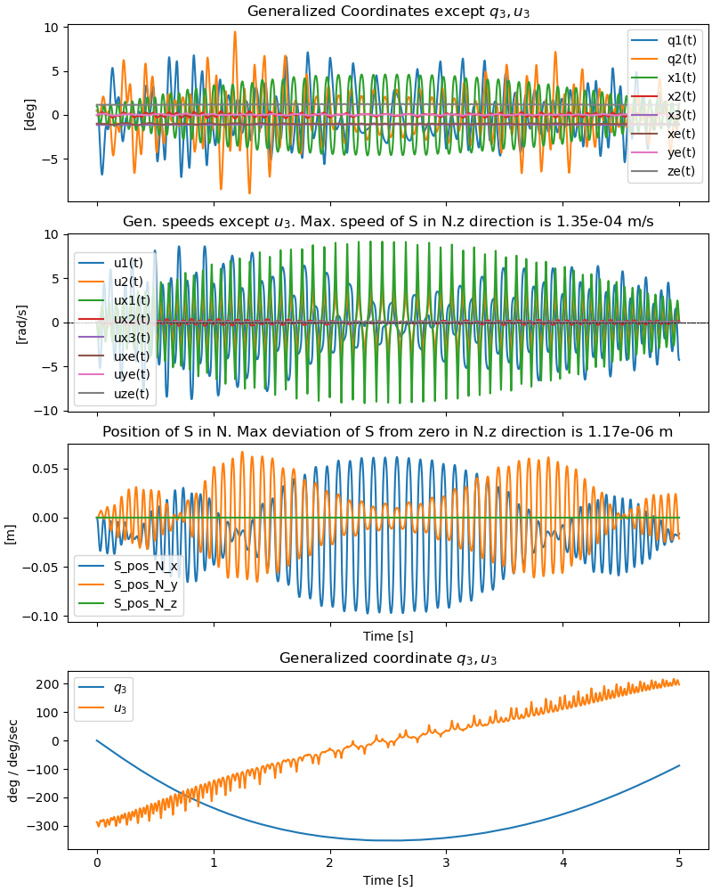
• \(q_1, q_2, q_3\) are the angles of the rattleback.

• \(u_1, u_2, u_3\) are the angular velocities of the rattleback.

• \(x_1, x_2, x_3\) are the coordinates of the contact point of the rattleback with the plane, in the body fixed frame.

• \(x_e, y_e, z_e\) are the coordinates of the geometric center of the rattleback in the inertial frame.

• \(u_{x1}, u_{x2}, u_{x3}\) are the velocities of the contact point of the rattleback with the plane, in the body fixed frame.

• \(u_{xe}, u_{ye}, u_{ze}\) are the velocities of the geometric center of the rattleback in the inertial frame.

Parameters

• \(m\) mass of the rattleback

• \(g\) gravitational acceleration

• \(a, b, c\) semi axes of the ellipsoid

• \(h\) distance geometric center to mass center

• \(A, B, C, D\) inertia parameters

import numpy as np
import sympy as sm
import sympy.physics.mechanics as me
import matplotlib.pyplot as plt
from matplotlib.collections import LineCollection
from scipy.integrate import solve_ivp
from pydy.system import System
from scipy.interpolate import CubicSpline
from matplotlib.animation import FuncAnimation

Kane’s Equations of Motion

N, R = sm.symbols('N, R', cls=me.ReferenceFrame)
O = me.Point('O')
Oe = me.Point('Oe')
t = me.dynamicsymbols._t
O.set_vel(N, 0)

The point S is the contact point of the rattleback with the plane. Ro is the center of mass of the rattleback.

S, Ro = sm.symbols('S, Ro', cls=me.Point)

Generalized coordinates and speeds.

q1, q2, q3, u1, u2, u3 = me.dynamicsymbols('q1, q2, q3, u1, u2, u3')
x1, x2, x3, ux1, ux2, ux3 = me.dynamicsymbols('x1, x2, x3, ux1, ux2, ux3')
xe, ye, ze, uxe, uye, uze = me.dynamicsymbols('xe, ye, ze, uxe, uye, uze')

Some parameters.

h, g, m, A, B, C, D = sm.symbols('h, g, m, A, B, C, D')
a, b, c = sm.symbols('a, b, c')
friktion = sm.symbols('friktion')

Orient the body fixed frame R. rot, rot1 are used for the kinematic differential equations.

R.orient_body_fixed(N, (q1, q2, q3), 'XYZ')
rot = R.ang_vel_in(N)
R.set_ang_vel(N, u1 * R.x + u2 * R.y + u3 * R.z)
rot1 = R.ang_vel_in(N)

Set the geometric center of the rattleback.

Oe.set_pos(O, xe * N.x + ye * N.y + ze * N.z)

Set the center of mass of the rattleback.

Ro.set_pos(Oe, -h * R.z)

Set the contact point of the rattleback with the plane and its velocity.

S.set_pos(Oe, x1*R.x + x2*R.y + x3*R.z)
S.set_vel(N, ux1*R.x + ux2*R.y + ux3*R.z)

Set the velocities of the geometric center and the center of mass of the rattleback. Here it is used that S has a no slip condition.

Oe.set_vel(N, R.ang_vel_in(N).cross(Oe.pos_from(S)))
Ro.set_vel(N, R.ang_vel_in(N).cross(Ro.pos_from(Oe)) + Oe.vel(N))

Define the rigid body of the rattleback.

inert = me.inertia(R, A, B, C, D, 0, 0)
rattleback = me.RigidBody('Rattleback', Ro, R, m, (inert, Ro))
bodies = [rattleback]

Forces and friction torques.

forces = [
        (Ro, -m * g * N.z),
        (R, -friktion * R.ang_vel_in(N))
    ]

This determines the location of the contact point S. It is from the a.m. paper and is the key to the whole simulation. The speed constraints are the time derivatives of the configuration constraints.

epsilon = -sm.sqrt((a * N.z.dot(R.x))**2 + (b * N.z.dot(R.y))**2 +
                   (c * N.z.dot(R.z))**2)

config_constr = sm.Matrix([
        x1 - (a**2 * N.z.dot(R.x) / epsilon),
        x2 - (b**2 * N.z.dot(R.y) / epsilon),
        x3 - (c**2 * N.z.dot(R.z) / epsilon)
    ])

speed_constr_S = config_constr.diff(t)

The speed constraints for the geometric center of the rattleback.

speed_constr_Oe = sm.Matrix([
        uxe - Oe.vel(N).dot(N.x),
        uye - Oe.vel(N).dot(N.y),
        uze - Oe.vel(N).dot(N.z)
])

Combine the speed constraints.

speed_constr = sm.Matrix([*speed_constr_S, *speed_constr_Oe])

Set up Kanes equations of motion.

q_ind = [q1, q2, q3, x1, x2, x3]
q_dep = [xe, ye, ze]
u_ind = [u1, u2, u3]
u_dep = [ux1, ux2, ux3, uxe, uye, uze]

kd = sm.Matrix([
    *[((rot - rot1).dot(uv)) for uv in N],
    x1.diff(t) - ux1,
    x2.diff(t) - ux2,
    x3.diff(t) - ux3,
    xe.diff(t) - uxe,
    ye.diff(t) - uye,
    ze.diff(t) - uze
])

kane = me.KanesMethod(
        N,
        q_ind,
        u_ind,
        q_dependent=q_dep,
        u_dependent=u_dep,
        kd_eqs=kd,
        configuration_constraints=config_constr,
        velocity_constraints=speed_constr,
)
fr, frstar = kane.kanes_equations(bodies, forces)

Define a special ode solver, needed here for accuracy.

def ode_solver(f, x0, ts, args=(), **kwargs):
    return solve_ivp(lambda t, x: f(x, t, *args), ts[[0, -1]], x0,
                     t_eval=ts, **kwargs).y.T

Define an instance of System.

sys = System(kane, ode_solver=ode_solver)

Set the parameters of the simulation.

sys.constants = {
    m: 1.0,                         # mass of the rattleback
    g: 9.81,                        # gravitational acceleration
    a: 0.2,                         # semi axes of the ellipsoid
    b: 0.03,                        # semi axes of the ellipsoid
    c: 0.02,                        # semi axes of the ellipsoid
    h: 0.01,                        # distance geometric center to mass center
    A: 2.e-4,                       # inertia parameters
    B: 1.6e-3,                      # inertia parameters
    C: 1.7e-3,                      # inertia parameters
    D: -2.0e-5,                     # inertia parameters
    friktion: 1.e-4,                # friction coefficient
    }

print('Constants of the system:')
for key, val in sys.constants.items():
    print(f'{key} = {val:.2e}')

Constants of the system:
m = 1.00e+00
g = 9.81e+00
a = 2.00e-01
b = 3.00e-02
c = 2.00e-02
h = 1.00e-02
A = 2.00e-04
B = 1.60e-03
C = 1.70e-03
D = -2.00e-05
friktion = 1.00e-04

Set the initial conditions of the independent coordinates and speeds.

sys.initial_conditions = {
    q1: np.deg2rad(0.5),        # initial orientation angles
    q2: np.deg2rad(0.5),
    q3: np.deg2rad(0.0),
    u1: 0.0,                     # initial angular velocities
    u2: 0.0,
    u3: -5.0,
}

Determine the initial conditions for the dependent coordinates and speeds, so that the constraints are satisfied. This is done by solving the constraints for the dependent coordinates and speeds, and then substituting the initial values of the independent coordinates and speeds, and the constants.

pL_pos = [key for key in sys.constants.keys()]
pL_vals = [sys.constants[key] for key in pL_pos]
qL = [q1, q2, q3, u1, u2, u3]
qL_vals = [sys.initial_conditions[key] for key in qL]

Pos of S in R as per D Levinson’s paper.

S_pos = sm.solve(config_constr, (x1, x2, x3))
S_pos_R = [S_pos[x1], S_pos[x2], S_pos[x3]]
S_pos_R_lam = sm.lambdify(qL + pL_pos, S_pos_R, cse=True)
x1_1, x2_1, x3_1 = S_pos_R_lam(*qL_vals, *pL_vals)
dict_S_pos = {x1: x1_1, x2: x2_1, x3: x3_1}

Speed of S in R.

speed_constr_S = speed_constr_S.subs({i.diff(t): j
                                      for i, j in zip(q_ind, u_ind + u_dep)})
S_speed_R = sm.solve(speed_constr_S, (ux1, ux2, ux3))
S_speed_R = [S_speed_R[ux1].subs(dict_S_pos),
             S_speed_R[ux2].subs(dict_S_pos),
             S_speed_R[ux3].subs(dict_S_pos)]
S_speed_R_lam = sm.lambdify(qL + pL_pos, S_speed_R, cse=True)
ux1_1, ux2_1, ux3_1 = S_speed_R_lam(*qL_vals, *pL_vals)
dict_S_speed_R = {ux1: ux1_1, ux2: ux2_1, ux3: ux3_1}

Initial conditons for Oe in N, so that S is at O initially. (Just convenience, any other point would be fine, too)

S_pos_N = sm.Matrix([S.pos_from(O).dot(N.x), S.pos_from(O).dot(N.y),
                     S.pos_from(O).dot(N.z)])

Oe_pos_N = sm.solve(S_pos_N, (xe, ye, ze))
Oe_pos_N = [Oe_pos_N[xe].subs(S_pos), Oe_pos_N[ye].subs(S_pos),
            Oe_pos_N[ze].subs(S_pos)]
Oe_pos_N_lam = sm.lambdify(qL + pL_pos, Oe_pos_N, cse=True)
xe1, ye1, ze1 = Oe_pos_N_lam(*qL_vals, *pL_vals)
dict_Oe_pos_N = {xe: xe1, ye: ye1, ze: ze1}

Initial conditions for Oe speed in N, so that S is at rest initially.

Oe_speed_N = sm.solve(speed_constr_Oe, (uxe, uye, uze))
Oe_speed_N = [me.msubs(Oe_speed_N[uxe], dict_Oe_pos_N, dict_S_pos),
              me.msubs(Oe_speed_N[uye], dict_Oe_pos_N, dict_S_pos),
              me.msubs(Oe_speed_N[uze], dict_Oe_pos_N, dict_S_pos)]
Oe_speed_N_lam = sm.lambdify(qL + pL_pos, Oe_speed_N)
uxe1, uye1, uze1 = Oe_speed_N_lam(*qL_vals, *pL_vals)
dict_Oe_speed_N = {uxe: uxe1, uye: uye1, uze: uze1}

Combine all initial conditions.

sys.initial_conditions = {**sys.initial_conditions, **dict_S_pos,
                          **dict_S_speed_R, **dict_Oe_pos_N,
                          **dict_Oe_speed_N}

print('Initial conditions:')
for key, val in sys.initial_conditions.items():
    print(f'{key} = {val:.4e}')

Initial conditions:
q1(t) = 8.7266e-03
q2(t) = 8.7266e-03
q3(t) = 0.0000e+00
u1(t) = 0.0000e+00
u2(t) = 0.0000e+00
u3(t) = -5.0000e+00
x1(t) = 1.7386e-02
x2(t) = -3.9120e-04
x3(t) = -1.9923e-02
ux1(t) = 8.6292e-02
ux2(t) = 1.9704e-03
ux3(t) = 7.3586e-04
xe(t) = -1.7212e-02
ye(t) = 2.1602e-04
ze(t) = 2.0076e-02
uxe(t) = 1.9559e-03
uye(t) = 8.6928e-02
uze(t) = 7.4154e-04

As generation='cython' and linear_sys_solver='numpy' are needed for speed, define the generator of the r.h.s here,

_ = sys.generate_ode_function(generator='cython', linear_sys_solver='numpy')

Numerical Integration

interval = 5.0
schritte = int(2000 * interval)
sys.times = np.linspace(0., interval, schritte)
times = sys.times

resultat = sys.integrate(method='DOP853', atol=1.e-12, rtol=1.e-12)
print('Shape of resultat', resultat.shape)

Shape of resultat (10000, 18)

Plot some Results

qL1 = q_ind + q_dep + u_ind + u_dep
bezeichnung = [str(i) for i in qL1]

S_vel_N = S.vel(N).subs({i.diff(t): j for i, j in zip(q_ind, u_ind + u_dep)})
S_vel_N = sm.Matrix([S_vel_N.dot(N.x), S_vel_N.dot(N.y), S_vel_N.dot(N.z)])
S_vel_N_lam = sm.lambdify(qL1 + pL_pos, S_vel_N, cse=True)
S_vel_N_np = np.zeros((resultat.shape[0], 3))
for i in range(resultat.shape[0]):
    S_vel_N_np[i] = S_vel_N_lam(*[resultat[i, j]
                                  for j in range(resultat.shape[1])],
                                *pL_vals).squeeze()

S_pos_N = [S.pos_from(O).dot(N.x), S.pos_from(O).dot(N.y),
           S.pos_from(O).dot(N.z)]
S_pos_N_lam = sm.lambdify(qL1 + pL_pos, S_pos_N, cse=True)
S_pos_np = np.zeros((resultat.shape[0], 3))
for i in range(resultat.shape[0]):
    S_pos_np[i] = S_pos_N_lam(*[resultat[i, j]
                                for j in range(resultat.shape[1])], *pL_vals)


fig, ax = plt.subplots(4, 1, figsize=(8, 10), constrained_layout=True,
                       sharex=True)

max_vel_S_z = np.max(np.abs(S_vel_N_np[:, 2]))
max_pos_S_z = np.max(np.abs(S_pos_np[:, 2]))

for i in (0, 1, 3, 4, 5, 6, 7, 8):
    ax[0].plot(sys.times, np.rad2deg(resultat[:, i]),
               label=f'{bezeichnung[i]}')
    ax[1].plot(sys.times, resultat[:, i+9], label=f'{bezeichnung[i+9]}')
    ax[1].axhline(0, color='k', lw=0.5, ls='--')

ax[0].set_ylabel('[deg]')
ax[0].set_title('Generalized Coordinates except $q_3, u_3$')
ax[1].set_ylabel('[rad/s]')
ax[1].set_title('Gen. speeds except $u_3$. Max. speed of S in N.z direction '
                f'is {max_vel_S_z:.2e} m/s')
ax[-1].set_xlabel('Time [s]')
ax[0].legend()
ax[1].legend()

koords = ['x', 'y', 'z']
for i in range(3):
    ax[2].plot(sys.times, S_pos_np[:, i], label=f'S_pos_N_{koords[i]}')
ax[2].set_ylabel('[m]')
ax[2].set_title('Position of S in N. Max deviation of S from zero in '
                f'N.z direction is {max_pos_S_z:.2e} m')
ax[2].set_xlabel('Time [s]')
_ = ax[2].legend()

ax[3].plot(sys.times, np.rad2deg(resultat[:, 2]), label='$q_3$')
ax[3].plot(sys.times, np.rad2deg(resultat[:, 11]), label='$u_3$')
ax[3].set_title('Generalized coordinate $q_3, u_3$')
ax[3].set_ylabel('deg / deg/sec')
_ = ax[3].legend()

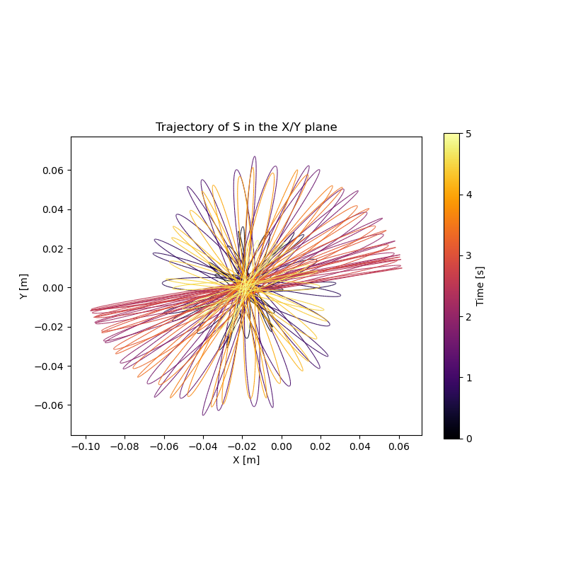
Plot the path of the contact point S.

fig, ax = plt.subplots(figsize=(8, 8))
min_x = np.min(S_pos_np[:, 0])
max_x = np.max(S_pos_np[:, 0])
min_y = np.min(S_pos_np[:, 1])
max_y = np.max(S_pos_np[:, 1])
ax.set_xlim(min_x - 0.01, max_x + 0.01)
ax.set_ylim(min_y - 0.01, max_y + 0.01)
ax.set_aspect('equal')
ax.set_xlabel('X [m]')
ax.set_ylabel('Y [m]')
ax.set_aspect('equal')
ax.set_title('Trajectory of S in the X/Y plane')

points = np.array([S_pos_np[:, 0], S_pos_np[:, 1]]).T.reshape(-1, 1, 2)
segments = np.concatenate([points[:-1], points[1:]], axis=1)

lc = LineCollection(segments, cmap='inferno',
                    norm=plt.Normalize(sys.times[0],
                                       sys.times[-1]))
lc.set_array(sys.times[:-1])   # color based on time
lc.set_linewidth(0.75)
ax.add_collection(lc)
cbar = plt.colorbar(lc, ax=ax, shrink=0.7)
cbar.set_label('Time [s]')

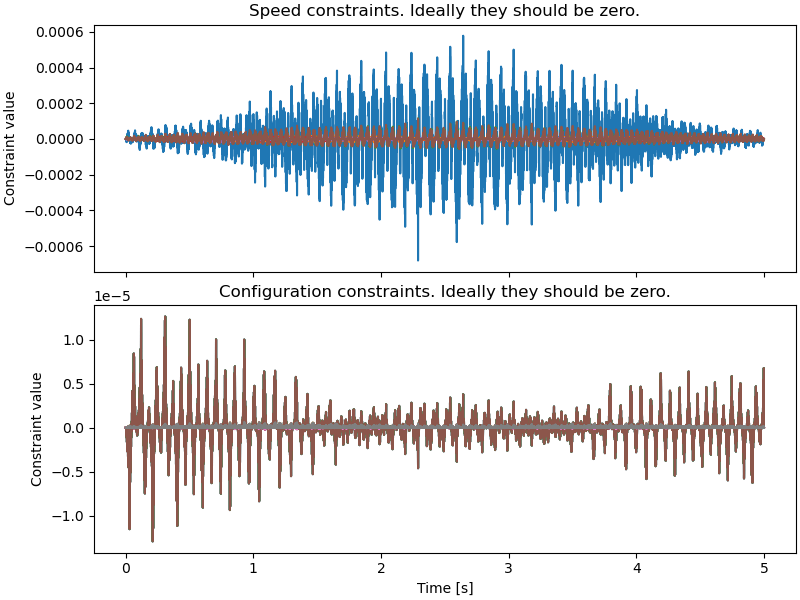
Check how well the constraints are satisfied.

speed_constraints = sys.evaluate_nonholonomic(x=resultat)
config_constraints = sys.evaluate_holonomic(x=resultat)

fig, ax = plt.subplots(2, 1, figsize=(8, 6), constrained_layout=True,
                       sharex=True)
for i in range(speed_constraints.shape[1]):
    ax[0].plot(sys.times, speed_constraints[:, i])
    ax[0].set_title('Speed constraints. Ideally they should be zero.')
    ax[0].set_ylabel('Constraint value')
    for i in range(config_constraints.shape[1]):
        ax[1].plot(sys.times, config_constraints[:, i])
    ax[1].set_title('Configuration constraints. Ideally they should be zero.')
    ax[1].set_xlabel('Time [s]')
    ax[1].set_ylabel('Constraint value')

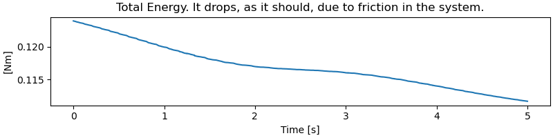
Plot the total energy of the system. It drops, as it should, due to friction in the system.

pot_energy = m * g * (Ro.pos_from(O).dot(N.z))
kin_energy = rattleback.kinetic_energy(N)
pot_lam = sm.lambdify(qL1 + pL_pos, pot_energy, cse=True)
kin_lam = sm.lambdify(qL1 + pL_pos, kin_energy, cse=True)

pot_np = np.empty(resultat.shape[0])
kin_np = np.empty(resultat.shape[0])
total_np = np.empty(resultat.shape[0])

for i in range(resultat.shape[0]):
    pot_np[i] = pot_lam(*resultat[i], *pL_vals)
    kin_np[i] = kin_lam(*resultat[i], *pL_vals)
    total_np[i] = pot_np[i] + kin_np[i]

fig2, ax2 = plt.subplots(1, 1, figsize=(8, 2), constrained_layout=True)
ax2.plot(sys.times, total_np)
ax2.set_ylabel('[Nm]')
ax2.set_title('Total Energy. It drops, as it should, '
              'due to friction in the system.')
_ = ax2.set_xlabel('Time [s]')

Animation

fps = 15
a2, b2, c2 = sys.constants[a], 4.5 * sys.constants[b], 4.5 * sys.constants[c]

t_arr = np.linspace(0.0, interval, schritte)
state_sol = CubicSpline(t_arr, resultat)

qL = q_ind + q_dep + u_ind + u_dep
coordinates = Oe.pos_from(O).to_matrix(N)
coordinates = coordinates.row_join(S.pos_from(O).to_matrix(N))
coords_lam = sm.lambdify(qL + pL_pos, coordinates, cse=True)

# Rotation matrices


def Rx(theta):
    return np.array([
        [1, 0, 0],
        [0, np.cos(theta), -np.sin(theta)],
        [0, np.sin(theta),  np.cos(theta)]
    ])


def Ry(theta):
    return np.array([
        [np.cos(theta), 0, np.sin(theta)],
        [0, 1, 0],
        [-np.sin(theta), 0, np.cos(theta)]
    ])


def Rz(theta):
    return np.array([
        [np.cos(theta), -np.sin(theta), 0],
        [np.sin(theta),  np.cos(theta), 0],
        [0, 0, 1]
    ])


def rotation_matrix(q1, q2, q3):
    # Change multiplication order if needed
    return Rz(q3) @ Ry(q2) @ Rx(q1)


# Create unit ellipsoid mesh
u = np.linspace(0, 2 * np.pi, 50)
v = np.linspace(0, np.pi, 30)

u, v = np.meshgrid(u, v)

X0 = a2 * np.cos(u) * np.sin(v)
Y0 = b2 * np.sin(u) * np.sin(v)
Z0 = c2 * np.cos(v)

points = np.vstack((X0.flatten(), Y0.flatten(), Z0.flatten()))

fig = plt.figure(figsize=(8, 8))
ax = fig.add_subplot(111, projection='3d')

ax.set_xlim(-0.25, 0.25)
ax.set_ylim(-0.25, 0.25)
ax.set_zlim(-0.25, 0.25)

ax.set_xlabel("X [m]", fontsize=15)
ax.set_ylabel("Y [m]", fontsize=15)
ax.set_zlabel("Z [m]", fontsize=15)
ax.set_title("Moving and Rotating Ellipsoid", fontsize=15)

# Initial plot
surface = [ax.plot_surface(X0, Y0, Z0, alpha=0.5, color='blue')]
contact_point, = ax.plot([0], [0], [0], color='black', markersize=8,
                         marker='o')
center_trail, = ax.plot([], [], [], color='black', linewidth=0.25)

# Create X/Y grid
x = np.linspace(-0.25, 0.25, 20)
y = np.linspace(-0.25, 0.25, 20)
X, Y = np.meshgrid(x, y)

# Z = 0 plane
Z = np.zeros_like(X)

# Draw the XY plane
ax.plot_surface(
    X, Y, Z,
    alpha=0.3,       # transparency
    color='yellow',
    edgecolor='none'
)


def update(t):
    global surface, contact_point, center_trail

    # Remove old surface
    surface[0].remove()

    msg = (f"Running time is {t:.2f} seconds, the animation is a bit "
           f"slow motion. \n The dot is the ocntact point, it is traced. \n "
           "The y / z coordinates of the ellipsoid are scaled up for better "
           "appearance.")
    ax.set_title(msg)

    # Center position
    M = coords_lam(*state_sol(t), *pL_vals)

    # Center trail
    x_trail, y_trail, z_trail = [], [], []
    for t_trail in sys.times[sys.times <= t]:
        M_trail = coords_lam(*state_sol(t_trail), *pL_vals)
        x_trail.append(M_trail[0, 1])
        y_trail.append(M_trail[1, 1])
        z_trail.append(M_trail[2, 1])
    center_trail.set_data(x_trail, y_trail)
    center_trail.set_3d_properties(z_trail)

    # Rotation
    q1, q2, q3 = state_sol(t)[:3]
    R = rotation_matrix(q1, q2, q3)

    # Rotate + translate
    rotated = R @ points
    X = rotated[0, :].reshape(X0.shape) + M[0, 0]
    Y = rotated[1, :].reshape(Y0.shape) + M[1, 0]
    Z = rotated[2, :].reshape(Z0.shape) + M[2, 0]

    # New surface
    surface[0] = ax.plot_surface(
        X, Y, Z,
        rstride=1,
        cstride=1,
        alpha=0.5,
        color='blue',
        linewidth=0.1,
        edgecolor='red',
    )

    contact_point.set_data([M[0, 1]], [M[1, 1]])
    contact_point.set_3d_properties([M[2, 1]])

    return surface[0], contact_point, center_trail


# Run animation
frames = np.linspace(0, interval, int(fps * (interval)))
ani = FuncAnimation(
    fig,
    update,
    frames=frames,
    interval=1500/fps,
    blit=False
)

plt.show()

Once Loop Reflect