Note
Go to the end to download the full example code.
Explorer Anomaly
Objectives
Show how to use some specific ode_solver
Show how to use
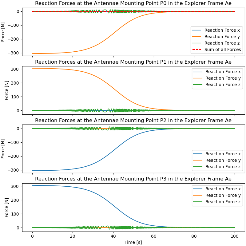
evaluate_odefor the calculation of the contributing forces (reaction forces) of the antennae to the explorer.
Description
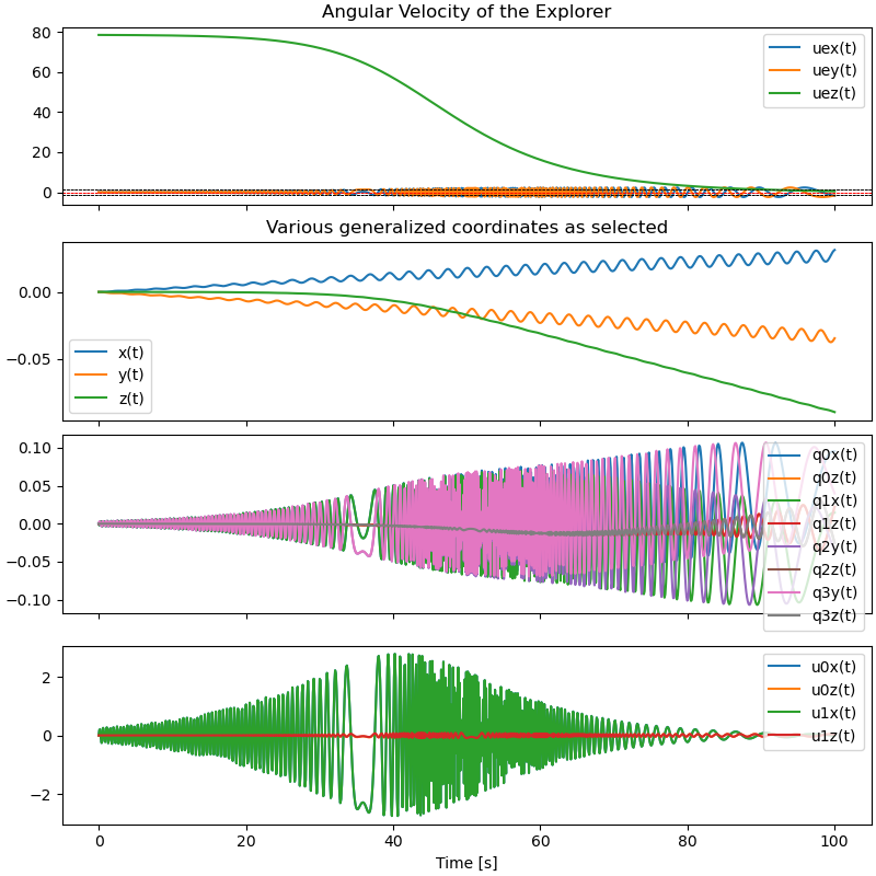
It is known, that for a rigid body the rotation around the axes of maximum or minimum moment of inertia is stable. Explorer1 showed, that the rotation around the axis of minimum moment of inertia may be unstable if the body is not rigid.
Many more details may be found here:
https://nescacademy.nasa.gov/video/cfbf4765ea984d05b2b5df46d2939ee11d which was also the inspiration for this example.
Here the explorer is modeled as a rigid body, a hollow tube. Four antennas are attached to the explorer via spherical joints. The antennas are modeled as thin rods. Their attachment points are located on a circumference near the center of gravity of the explorer, evenly spaced. Their neutral direction is normal to the surface of the explorer at the points of attachment. When they are deflected from their neutral position, a restoring torque acts on them, proportional to the deflection angle and a damping torque, proportional to the angular velocity, with constants \(k_\textrm{{torque}}\) and \(\mu_\textrm{{torque}}\). The opposite torque acts on the explorer.
As this takes place in outer space no gravity is present.
Notes
The dimensions and the masses of the explorer and the antennas are, as well as the constants \(k_\textrm{{torque}}\) and \(\mu_\textrm{{torque}}\) are courtesy Dr. David Levinson via Dr. Carlos Roithmayr.
The equations of motion are derived using Kane’s method.
As there is dampening, the total energy of the system decreases.
As there are no external forces or torques, the angular momentum of the system must be constant.
The animation is difficult: At first the motion is very fast, then it slows down substantially. Due to space limitation just a few parts are shown.
While pydy version 0.9.4 is the latest release, the developmental version of pydy must be used.
States
\(x, y, z\) : Position of the center of gravity of the explorer in the inertial frame
\(u_x, u_y, u_z\) : Velocity of the center of gravity of the explorer in the inertial frame
\(q_{ex}, q_{ey}, q_{ez}\) : Orientation of the body fixed frame of the explorer
\(u_{ex}, u_{ey}, u_{ez}\) : Angular velocity of the body fixed frame of the explorer
\(q_{0x}, q_{0z}\) : Orientation of the body fixed frame of antenna 0
\(u_{0x}, u_{0z}\) : Angular velocity of the body fixed frame of antenna 0
\(q_{1x}, q_{1z}\) : Orientation of the body fixed frame of antenna 1
\(u_{1x}, u_{1z}\) : Angular velocity of the body fixed frame of antenna 1
\(q_{2y}, q_{2z}\) : Orientation of the body fixed frame of antenna 2
\(u_{2y}, u_{2z}\) : Angular velocity of the body fixed frame of antenna 2
\(q_{3y}, q_{3z}\) : Orientation of the body fixed frame of antenna 3
\(u_{3y}, u_{3z}\) : Angular velocity of the body fixed frame of antenna 3
Parameters
\(m_e\) : Mass of the explorer
\(m_a\) : Mass of each antenna
\(r_{ei}\) : Inner radius of the explorer
\(r_{eo}\) : Outer radius of the explorer
\(L_e\) : Length of the explorer
\(L_a\) : Length of each antenna
\(\textrm{dist}\) : Distance of the attachment points of the antennas from the center of gravity of the explorer in radial direction
\(\textrm{shift}\) : Location of the attachment points of the antennas in the axial direction from the center of gravity of the explorer
\(k_\textrm{{torque}}\) : Spring constant
\(\mu_\textrm{{torque}}\) : Damping constant
import numpy as np
import sympy as sm
import matplotlib.pyplot as plt
import sympy.physics.mechanics as me
from scipy.integrate import solve_ivp
from scipy.optimize import root
from scipy.interpolate import CubicSpline
from pydy.system import System
from mpl_toolkits.mplot3d import Axes3D # noqa: F401
from matplotlib import animation
Equations of Motion, Kane’s Method
N, Ae, Aa0, Aa1, Aa2, Aa3 = sm.symbols('N Ae Aa0 Aa1 Aa2 Aa3',
cls=me.ReferenceFrame)
O = me.Point('O')
O.set_vel(N, 0)
t = me.dynamicsymbols._t
Points where the antennae attach to the explorer.
P0, P1, P2, P3 = sm.symbols('P0 P1 P2 P3', cls=me.Point)
Mass centers of the explorer and antennae.
Aoe, Aoa0, Aoa1, Aoa2, Aoa3 = sm.symbols('Aoe Aoa0 Aoa1 Aoa2 Aoa3',
cls=me.Point)
Coordinates of the mass center of the explorer.
x, y, z, ux, uy, uz = me.dynamicsymbols('x, y, z, ux, uy, uz')
Coordinates of body fixed frame of the explorer.
qex, qey, qez = me.dynamicsymbols('qex, qey, qez')
uex, uey, uez = me.dynamicsymbols('uex, uey, uez')
# %%
# Coordinates of the body fixed frames of the antennae.
q0x, q0z, u0x, u0z = me.dynamicsymbols('q0x, q0z, u0x, u0z')
q1x, q1z, u1x, u1z = me.dynamicsymbols('q1x, q1z, u1x, u1z')
q2y, q2z, u2y, u2z = me.dynamicsymbols('q2y, q2z, u2y, u2z')
q3y, q3z, u3y, u3z = me.dynamicsymbols('q3y, q3z, u3y, u3z')
aux0x, aux0y, aux0z, f0x, f0y, f0z = me.dynamicsymbols(
'aux0x, aux0y, aux0z, f0x, f0y, f0z')
aux1x, aux1y, aux1z, f1x, f1y, f1z = me.dynamicsymbols(
'aux1x, aux1y, aux1z, f1x, f1y, f1z')
aux2x, aux2y, aux2z, f2x, f2y, f2z = me.dynamicsymbols(
'aux2x, aux2y, aux2z, f2x, f2y, f2z')
aux3x, aux3y, aux3z, f3x, f3y, f3z = me.dynamicsymbols(
'aux3x, aux3y, aux3z, f3x, f3y, f3z')
Place holders for the u_i.diff(t) in the reaction forces.
rhs_list = [sm.symbols('rhs' + str(i)) for i in range(14)]
m_e, m_a, rei, reo, shift, La, Le, dist = sm.symbols(
'm_e m_a rei reo shift La Le dist')
k_torque, mu_torque = sm.symbols('k_torque mu_torque')
rot, rot1 for the kinematical differential equations.
rot, rot1 = [], []
Explorer body frame.
Ae.orient_body_fixed(N, (qex, qey, qez), 'XYZ')
rot.append(Ae.ang_vel_in(N))
Ae.set_ang_vel(N, uex*Ae.x + uey*Ae.y + uez*Ae.z)
rot1.append(Ae.ang_vel_in(N))
Antenna 0 body frame.
Aa0.orient_body_fixed(Ae, (q0x, 0, q0z), 'XYZ')
rot.append(Aa0.ang_vel_in(N))
Aa0.set_ang_vel(Ae, u0x*Aa0.x + u0z*Aa0.z)
rot1.append(Aa0.ang_vel_in(N))
Antenna 1 body frame.
Aa1.orient_body_fixed(Ae, (q1x, 0, q1z), 'XYZ')
rot.append(Aa1.ang_vel_in(N))
Aa1.set_ang_vel(Ae, u1x*Aa1.x + u1z*Aa1.z)
rot1.append(Aa1.ang_vel_in(N))
Antenna 2 body frame.
Aa2.orient_body_fixed(Ae, (0, q2y, q2z), 'XYZ')
rot.append(Aa2.ang_vel_in(N))
Aa2.set_ang_vel(Ae, u2y*Aa2.y + u2z*Aa2.z)
rot1.append(Aa2.ang_vel_in(N))
Antenna 3 body frame.
Aa3.orient_body_fixed(Ae, (0, q3y, q3z), 'XYZ')
rot.append(Aa3.ang_vel_in(N))
Aa3.set_ang_vel(Ae, u3y*Aa3.y + u3z*Aa3.z)
rot1.append(Aa3.ang_vel_in(N))
Center of gravity of explorer.
Aoe.set_pos(O, x*N.x + y*N.y + z*N.z)
Aoe.set_vel(N, ux*N.x + uy*N.y + uz*N.z)
Points where the antennae attach to the explorer.
P0.set_pos(Aoe, dist*Ae.y + shift*Ae.z)
vP0 = P0.v2pt_theory(Aoe, N, Ae)
P0.set_vel(N, vP0 + aux0x*Ae.x + aux0y*Ae.y + aux0z*Ae.z)
P1.set_pos(Aoe, -dist*Ae.y + shift*Ae.z)
vP1 = P1.v2pt_theory(Aoe, N, Ae)
P1.set_vel(N, vP1 + aux1x*Ae.x + aux1y*Ae.y + aux1z*Ae.z)
P2.set_pos(Aoe, dist*Ae.x + shift*Ae.z)
vP2 = P2.v2pt_theory(Aoe, N, Ae)
P2.set_vel(N, vP2 + aux2x*Ae.x + aux2y*Ae.y + aux2z*Ae.z)
P3.set_pos(Aoe, -dist*Ae.x + shift*Ae.z)
vP3 = P3.v2pt_theory(Aoe, N, Ae)
P3.set_vel(N, vP3 + aux3x*Ae.x + aux3y*Ae.y + aux3z*Ae.z)
Set the mass centers of the antennae.
Aoa0.set_pos(P0, La/2 * Aa0.y)
Aoa0.v2pt_theory(P0, N, Aa0)
Aoa1.set_pos(P1, -La/2 * Aa1.y)
Aoa1.v2pt_theory(P1, N, Aa1)
Aoa2.set_pos(P2, La/2 * Aa2.x)
Aoa2.v2pt_theory(P2, N, Aa2)
Aoa3.set_pos(P3, -La/2 * Aa3.x)
_ = Aoa3.v2pt_theory(P3, N, Aa3)
Set the torques on the antennae.
torque0x = -(k_torque * q0x + mu_torque * u0x) * Aa0.x
torque0z = - (k_torque * q0z + mu_torque * u0z) * Aa0.z
torque1x = -(k_torque * q1x + mu_torque * u1x) * Aa1.x
torque1z = - (k_torque * q1z + mu_torque * u1z) * Aa1.z
torque2y = -(k_torque * q2y + mu_torque * u2y) * Aa2.y
torque2z = -(k_torque * q2z + mu_torque * u2z) * Aa2.z
torque3y = -(k_torque * q3y + mu_torque * u3y) * Aa3.y
torque3z = - (k_torque * q3z + mu_torque * u3z) * Aa3.z
torques = [
(Aa0, torque0x + torque0z),
(Aa1, torque1x + torque1z),
(Aa2, torque2y + torque2z),
(Aa3, torque3y + torque3z),
# Reaction torque on explorer
(Ae, -(torque0x + torque0z + torque1x + torque1z +
torque2y + torque2z + torque3y + torque3z)),
# for the reaction forces.
(P0, f0x*Ae.x + f0y*Ae.y + f0z*Ae.z),
(P1, f1x*Ae.x + f1y*Ae.y + f1z*Ae.z),
(P2, f2x*Ae.x + f2y*Ae.y + f2z*Ae.z),
(P3, f3x*Ae.x + f3y*Ae.y + f3z*Ae.z),
]
Bodies and their inertias. Explorer is a hollow tube.
iXXe = m_e/12 * (3*(rei**2 + reo**2) + Le**2)
iZZe = m_e/2 * (rei**2 + reo**2)
iYYe = iXXe
Inertia_e = me.inertia(Ae, iXXe, iYYe, iZZe)
explorer1 = me.RigidBody('explorer1', Aoe, Ae, m_e, (Inertia_e, Aoe))
antennea are rods.
iRR = 1/12*m_a*La**2
inertia_0 = me.inertia(Aa0, iRR, 0, iRR)
link0 = me.RigidBody('link0', Aoa0, Aa0, m_a, (inertia_0, Aoa0))
inertia_1 = me.inertia(Aa1, iRR, 0, iRR)
link1 = me.RigidBody('link1', Aoa1, Aa1, m_a, (inertia_1, Aoa1))
inertia_2 = me.inertia(Aa2, 0, iRR, iRR)
link2 = me.RigidBody('link2', Aoa2, Aa2, m_a, (inertia_2, Aoa2))
inertia_3 = me.inertia(Aa3, 0, iRR, iRR)
link3 = me.RigidBody('link3', Aoa3, Aa3, m_a, (inertia_3, Aoa3))
bodies = [explorer1, link0, link1, link2, link3]
q_ind = [x, y, z, qex, qey, qez, q0x, q0z, q1x, q1z, q2y, q2z, q3y, q3z]
u_ind = [ux, uy, uz, uex, uey, uez, u0x, u0z, u1x, u1z, u2y, u2z, u3y, u3z]
aux = [aux0x, aux0y, aux0z,
aux1x, aux1y, aux1z,
aux2x, aux2y, aux2z,
aux3x, aux3y, aux3z]
F_r = [f0x, f0y, f0z,
f1x, f1y, f1z,
f2x, f2y, f2z,
f3x, f3y, f3z]
kd = sm.Matrix([
ux - x.diff(t),
uy - y.diff(t),
uz - z.diff(t),
*[(rot[0] - rot1[0]).dot(uv) for uv in Ae],
*[(rot[1] - rot1[1]).dot(uv) for uv in (Aa0.x, Aa0.z)],
*[(rot[2] - rot1[2]).dot(uv) for uv in (Aa1.x, Aa1.z)],
*[(rot[3] - rot1[3]).dot(uv) for uv in (Aa2.y, Aa2.z)],
*[(rot[4] - rot1[4]).dot(uv) for uv in (Aa3.y, Aa3.z)],
])
kane = me.KanesMethod(
N,
q_ind,
u_ind,
kd,
u_auxiliary=aux,
)
fr, frstar = kane.kanes_equations(bodies, torques)
eingepraegt = kane.auxiliary_eqs.subs({i.diff(t): rhs_list[j]
for j, i in enumerate(u_ind)})
Energy and Angular Momentum.
aux_dict = {i: 0 for i in aux}
kin_energy = sum([b.kinetic_energy(N).subs(aux_dict) for b in bodies])
spring_energy = 0.5 * k_torque * (q0x**2 + q0z**2 + q1x**2 + q1z**2 +
q2y**2 + q2z**2 + q3y**2 + q3z**2)
ang_momentum = [
sum([body.angular_momentum(O, N).dot(N.x).subs(aux_dict)
for body in bodies]),
sum([body.angular_momentum(O, N).dot(N.y).subs(aux_dict)
for body in bodies]),
sum([body.angular_momentum(O, N).dot(N.z).subs(aux_dict)
for body in bodies]),
]
Define a specific ode solver.
def ode_solver(f, x0, ts, args=(), **kwargs):
return solve_ivp(lambda t, x: f(x, t, *args), ts[[0, -1]], x0,
t_eval=ts, **kwargs).y.T
Initialize System.
sys = System(kane, ode_solver=ode_solver)
Define the constants of the system.
sys.constants = {
Le: 2.05,
rei: 0.060,
reo: 0.076,
dist: 0.076,
La: 0.56,
m_e: 13.9,
m_a: 13.9 / 100.0,
shift: 0.1,
k_torque: 0.565,
mu_torque: 1.13,
}
Set the initial_conditions.
sys.initial_conditions = {
x: 0.0,
y: 0.0,
z: 0.0,
ux: 0.0,
uy: 0.0,
uz: 0.0,
qex: 0.0,
qey: 0.0,
qez: 0.0,
uez: 750.0 * 2 * np.pi / 60, # 750 rpm
uex: 750.0 / 1.e3,
uey: 750.0 / 1.e3,
q0x: 0.0,
q0z: 0.0,
u0x: 0.0,
u0z: 0.0,
q1x: 0.0,
q1z: 0.0,
u1x: 0.0,
u1z: 0.0,
q2y: 0.0,
q2z: 0.0,
u2y: 0.0,
u2z: 0.0,
q3y: 0.0,
q3z: 0.0,
u3y: 0.0,
u3z: 0.0,
}
In the force vector are the reaction forces and the virtual speeds. As they do no work, they are set to zero. This is not really necessary as System() will do this automatically, but it is done here for clarity.
spec_sym = sys.specifieds_symbols
sys.specifieds = {'symbols': spec_sym, 'values': np.zeros(12)}
As speed is of no concern here, lambdify is used.
qL = q_ind + u_ind
pL = [key for key in sys.constants.keys()]
pL_vals = [sys.constants[key] for key in pL]
kin_lam = sm.lambdify(qL + pL, kin_energy, cse=True)
spring_lam = sm.lambdify(qL + pL, spring_energy, cse=True)
ang_momentum_lam = sm.lambdify(qL + pL, ang_momentum, cse=True)
eingepraegt_lam = sm.lambdify(F_r + qL + pL + rhs_list,
eingepraegt, cse=True)
Numerical Integration
Ensure that for speed the cython generator is used and the linear system solver is numpy. This is to get an efficient r.h.s. for the numerical integration.
_ = sys.generate_ode_function(generator='cython', linear_sys_solver='numpy')
Set the integration interval and the point of time where the result is returned.
sys.times = np.linspace(0., 100.0, 2000)
Set the kwargs of solve_ivp used in the ode_solver.
resultat = sys.integrate(method='DOP853', atol=1.e-9, rtol=1.e-9)
print('resultat shape', resultat.shape)
resultat shape (2000, 28)
Plot some generalized coordinates.
bezeichnung = [str(i) for i in q_ind + u_ind]
fig, ax = plt.subplots(4, 1, figsize=(8, 9), layout='constrained',
sharex=True)
for i in (17, 18, 19):
begin = 0
ax[0].plot(sys.times[begin: resultat.shape[0]], resultat[begin:, i],
label=bezeichnung[i])
ax[0].axhline(1.35, color='black', lw=0.5, ls='--')
ax[0].axhline(-1.35, color='black', lw=0.5, ls='--')
ax[0].axhline(0.0, color='red', lw=0.5, ls='--')
ax[0].set_title('Angular Velocity of the Explorer')
ax[0].set_ylabel('Angular Velocity [rad/s]')
_ = ax[0].legend()
for i in (0, 1, 2):
ax[1].plot(sys.times[begin: resultat.shape[0]], resultat[begin:, i],
label=bezeichnung[i])
ax[1].set_title('Position of the center of gravity of the explorer')
ax[1].set_ylabel('Position [m]')
_ = ax[1].legend()
for i in (6, 7, 8, 9, 10, 11, 12, 13):
ax[2].plot(sys.times[begin: resultat.shape[0]],
np.rad2deg(resultat[begin:, i]),
label=bezeichnung[i])
ax[2].set_title('Orientation of the Antennae, zero is the position normal '
'to the surface of the explorer')
ax[2].set_ylabel('Orientation [deg]')
_ = ax[2].legend()
for i in (20, 21, 22, 23):
ax[3].plot(sys.times[begin: resultat.shape[0]], resultat[begin:, i],
label=bezeichnung[i])
ax[3].set_title('Angular Velocity of the Antennae')
ax[3].set_ylabel('Angular Velocity [rad/s]')
ax[-1].set_xlabel('Time [s]')
_ = ax[3].legend()
Plot Energy and Angular Momentum
fig, ax = plt.subplots(2, 1, figsize=(8, 4), layout='constrained', sharex=True)
kin_np = kin_lam(*(resultat.T), *pL_vals)
spring_np = spring_lam(*(resultat.T), *pL_vals)
total_np = kin_np + spring_np
begin = 0
ax[0].plot(sys.times[begin: resultat.shape[0]], kin_np[begin:],
label='kinetic energy')
ax[0].plot(sys.times[begin: resultat.shape[0]], spring_np[begin:],
label='spring energy')
ax[0].plot(sys.times[begin: resultat.shape[0]], total_np[begin:],
label='total energy')
ax[0].set_ylabel('Energy [J]')
ax[0].set_title('Energy of the system')
_ = ax[0].legend()
max_x = np.max(ang_momentum_lam(*(resultat.T), *pL_vals)[0])
may_y = np.max(ang_momentum_lam(*(resultat.T), *pL_vals)[1])
max_z = np.max(ang_momentum_lam(*(resultat.T), *pL_vals)[2])
min_x = np.min(ang_momentum_lam(*(resultat.T), *pL_vals)[0])
min_y = np.min(ang_momentum_lam(*(resultat.T), *pL_vals)[1])
min_z = np.min(ang_momentum_lam(*(resultat.T), *pL_vals)[2])
max_mom = max_x + may_y + max_z
min_mon = min_x + min_y + min_z
error = (max_mom - min_mon) / max_mom
print(f'Max error from conservation of angular momentum: {error:.3e}')
for i, j in enumerate(['x', 'y', 'z']):
ax[1].plot(sys.times[: resultat.shape[0]], ang_momentum_lam(
*(resultat.T), *pL_vals)[i], label=f'angular momentum {j}')
ax[1].set_ylabel('Angular momentum [kg m²/s]')
ax[1].set_title('Angular momentum of the system')
_ = ax[1].legend()
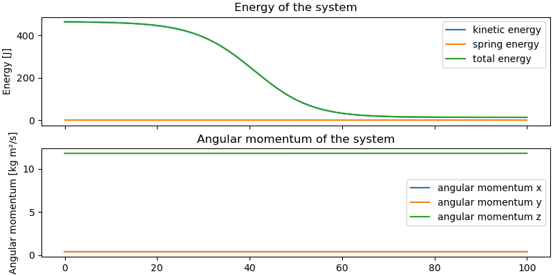
Max error from conservation of angular momentum: 8.853e-03
Calculate Reaction Forces on Points, where the Antennas are attached to Explorer
RHS = sys.evaluate_ode(x=resultat)
reaction_forces = np.empty((resultat.shape[0], 12))
summe_np = np.empty(resultat.shape[0])
def func_react(x0, args):
return eingepraegt_lam(*x0, *args).squeeze()
x0 = np.array([0.0 for _ in range(len(F_r))])
for i in range(resultat.shape[0]):
args = np.array([*resultat[i, :], *pL_vals, *RHS[i, 14:]])
loesung = root(func_react, x0, args=args)
reaction_forces[i, :] = loesung.x
x0 = loesung.x
summe_np[i] = np.sum(loesung.x)
begin = 0
fig, ax = plt.subplots(4, 1, figsize=(8, 8), layout='constrained',
sharex=True)
for i in range(4):
for k, j in zip(reaction_forces[:, 3*i:3*i+3].T, ('x', 'y', 'z')):
ax[i].plot(sys.times[begin:], k[begin:], label=f'Reaction Force {j}')
ax[i].set_ylabel('Force [N]')
ax[i].set_title(f'Reaction Forces at the Antennae Mounting Point P{i} '
'in the Explorer Frame Ae')
ax[i].legend()
_ = ax[-1].set_xlabel('Time [s]')
ax[0].plot(sys.times[begin:], summe_np[begin:], 'r--',
label='Sum of all Forces')
_ = ax[0].legend()
Animation using PyDy Visualization
# In this sphinx environment the animation does not work. The program was left
# here to show the simplicity of the animation with PyDy Visualization compared
# to Matplotlib.
# from pydy.viz.shapes import Cylinder, Sphere
# from pydy.viz.scene import Scene
# from pydy.viz.visualization_frame import VisualizationFrame
#
# Define the right frames so the cylinders point in the Y direction
# Be, Ba0, Ba1, Ba2, Ba3 = sm.symbols('Be B0 B1 B2 B3', cls=me.ReferenceFrame)
# Point to see easily how explorer is turning.
# P_red = me.Point('P_red')
# Be.orient_body_fixed(Ae, (-np.pi/2, 0, 0), 'XYZ')
# Ba1.orient_body_fixed(Aa1, (0, 0, np.pi), 'XYZ')
# Ba2.orient_body_fixed(Aa2, (0, 0, np.pi/2), 'XYZ')
# Ba3.orient_body_fixed(Aa3, (0, 0, -np.pi/2), 'XYZ')
# P_red.set_pos(Aoe, Le/4 * Be.y + reo * Be.z)
# farben = ['grey', 'blue', 'green', 'red', 'yellow']
# viz_frames = []
# mass_centers = [Aoe, Aoa0, Aoa1, Aoa2, Aoa3]
# frames = [Ae, Aa0, Ba1, Ba2, Ba3]
# for i, antenna in enumerate(bodies[1:]):
# antenna_shape = Cylinder(name='antenna{}'.format(i),
# radius=0.025,
# length=sys.constants[La],
# color=farben[i])
# viz_frames.append(VisualizationFrame('antenna_frame{}'.format(i),
# frames[i+1],
# mass_centers[i+1],
# antenna,
# antenna_shape))
# explorer_shape = Cylinder(name='explorer',
# radius=sys.constants[reo],
# length=sys.constants[Le],
# color=farben[0])
# viz_frames.append(VisualizationFrame('explorer_frame',
# Be,
# mass_centers[0],
# explorer1,
# explorer_shape))
# P_red_shape = Sphere(name='red_sphere',
# radius=0.05,
# color='red')
# viz_frames.append(VisualizationFrame('red_sphere_frame',
# Be,
# P_red,
# P_red,
# P_red_shape))
# scene = Scene(N, O, *viz_frames)
# Provide the data to compute the trajectories of the visualization frames.
# scene.times = sys. times
# scene.constants = dict(zip(pL, pL_vals))
# scene.states_symbols = q_ind + u_ind
# scene.states_trajectories = resultat
# scene.display_jupyter(axes_arrow_length=20)
Animation with Matplotlib
fps = 1
# Create the end points of the antennas
P01, P11, P21, P31, omega = sm.symbols('P01 P11 P21 P31 omega', cls=me.Point)
P01.set_pos(P0, sys.constants[La] * Aa0.y)
P11.set_pos(P1, -sys.constants[La] * Aa1.y)
P21.set_pos(P2, sys.constants[La] * Aa2.x)
P31.set_pos(P3, -sys.constants[La] * Aa3.x)
omega.set_pos(Aoe, uex*Ae.x + uey*Ae.y + uez*Ae.z)
coordinates = Aoe.pos_from(O).to_matrix(N)
for point in (P0, P01, P1, P11, P2, P21, P3, P31):
coordinates = coordinates.row_join(point.pos_from(O).to_matrix(N))
coordinates = coordinates.row_join(omega.pos_from(Aoe).to_matrix(N))
coordinates_lam = sm.lambdify(qL + pL, coordinates, cse=True)
t_arr = sys.times
state_sol = CubicSpline(t_arr, resultat)
# cylinder generation
def make_cylinder_mesh(Le, reo, n_theta=48, n_z=10):
# Create a cylinder mesh centered at origin along the z-axis:
# - z in [-Le/2, +Le/2]
# - radius = reo
# Returns X,Y,Z arrays shaped (n_z, n_theta)
theta = np.linspace(0, 2*np.pi, n_theta)
z = np.linspace(-Le/2, Le/2, n_z)
Theta, Z = np.meshgrid(theta, z)
X = reo * np.cos(Theta)
Y = reo * np.sin(Theta)
return X, Y, Z
# Rotation matrices
def Rx(angle):
c, s = np.cos(angle), np.sin(angle)
return np.array([[1, 0, 0],
[0, c, -s],
[0, s, c]])
def Ry(angle):
c, s = np.cos(angle), np.sin(angle)
return np.array([[c, 0, s],
[0, 1, 0],
[-s, 0, c]])
def Rz(angle):
c, s = np.cos(angle), np.sin(angle)
return np.array([[c, -s, 0],
[s, c, 0],
[0, 0, 1]])
# Apply transform
def transform_cylinder(X, Y, Z, Aoe, qx, qy, qz):
# Apply rotation (qx,qy,qz) and translation Aoe to the mesh.
# Rotation order: Rx then Ry then Rz => R = Rz @ Ry @ Rx
# flatten points for matrix multiplication
pts = np.vstack((X.ravel(), Y.ravel(), Z.ravel())) # shape (3, N)
# Build rotation matrix according to selected convention
R = Rz(qz) @ Ry(qy) @ Rx(qx)
pts_rot = R @ pts
pts_rot[0, :] += Aoe[0]
pts_rot[1, :] += Aoe[1]
pts_rot[2, :] += Aoe[2]
Xr = pts_rot[0, :].reshape(X.shape)
Yr = pts_rot[1, :].reshape(Y.shape)
Zr = pts_rot[2, :].reshape(Z.shape)
return Xr, Yr, Zr
def init():
Le1 = sys.constants[Le] # length
reo1 = sys.constants[reo] # radius
X, Y, Z = make_cylinder_mesh(Le1, reo1, n_theta=16, n_z=8)
fig = plt.figure(figsize=(8, 8))
ax = fig.add_subplot(111, projection='3d')
ax.set_box_aspect([1, 1, 1]) # make aspect equal
L = 1.5
ax.set_xlim(-L, L)
ax.set_ylim(-L, L)
ax.set_zlim(-L, L)
ax.set_xlabel('X [m]', fontsize=15)
ax.set_ylabel('Y [m]', fontsize=15)
ax.set_zlabel('Z [m]', fontsize=15)
# initial pose
coords = coordinates_lam(*state_sol(0), *pL_vals)
Aoe0 = np.array([coords[0, 0], coords[1, 0], coords[2, 0]])
qx0, qy0, qz0 = state_sol(0)[3:6] # explorer angles
Xr, Yr, Zr = transform_cylinder(X, Y, Z, Aoe0, qx0, qy0, qz0)
surf = ax.plot_surface(Xr, Yr, Zr, rstride=2, cstride=2, linewidth=0,
alpha=0.7, color='grey')
antenna0, = ax.plot([], [], [], color='black', lw=2)
antenna1, = ax.plot([], [], [], color='black', lw=2)
antenna2, = ax.plot([], [], [], color='black', lw=2)
antenna3, = ax.plot([], [], [], color='black', lw=2)
pfeil1 = ax.quiver(coords[0, 0], coords[1, 0], coords[2, 0],
coords[0, 9],
coords[1, 9],
coords[2, 9],
color='red',
arrow_length_ratio=0.3,)
return (fig, ax, surf, antenna0, antenna1, antenna2, antenna3, pfeil1,
X, Y, Z)
fig, ax, surf, antenna0, antenna1, antenna2, antenna3, pfeil1, X, Y, Z = init()
def update(t):
global surf, pfeil1
# remove previous surface and omega
surf.remove()
pfeil1.remove()
ax.set_title(f"Running time: {t:.2f} sec \n The red arrow shows the "
f"direction and magnitude of the angular velocity \n "
f"vector of the explorer", fontsize=12)
coords = coordinates_lam(*state_sol(t), *pL_vals)
# create explorer
Aoe = np.array([coords[0, 0], coords[1, 0], coords[2, 0]])
qx, qy, qz = state_sol(t)[3:6] # explorer angles
Xr, Yr, Zr = transform_cylinder(X, Y, Z, Aoe, qx, qy, qz)
surf = ax.plot_surface(Xr, Yr, Zr, rstride=2, cstride=2, linewidth=0,
alpha=0.8, color='grey')
antenna0.set_data([coords[0, 1], coords[0, 2]],
[coords[1, 0], coords[1, 1]])
antenna0.set_3d_properties([coords[2, 0], coords[2, 1]])
antenna1.set_data([coords[0, 3], coords[0, 4]],
[coords[1, 3], coords[1, 4]])
antenna1.set_3d_properties([coords[2, 3], coords[2, 4]])
antenna2.set_data([coords[0, 5], coords[0, 6]],
[coords[1, 5], coords[1, 6]])
antenna2.set_3d_properties([coords[2, 5], coords[2, 6]])
antenna3.set_data([coords[0, 7], coords[0, 8]],
[coords[1, 7], coords[1, 8]])
antenna3.set_3d_properties([coords[2, 7], coords[2, 8]])
scale_factor = 0.025
pfeil1 = ax.quiver(coords[0, 0], coords[1, 0], coords[2, 0],
scale_factor * coords[0, 9],
scale_factor * coords[1, 9],
scale_factor * coords[2, 9],
color='red', arrow_length_ratio=0.2)
return surf, antenna0, antenna1, antenna2, antenna3, pfeil1
frames = np.concatenate((sys.times[: 25], sys.times[1000: 1050],
sys.times[1975:]))
ani = animation.FuncAnimation(fig, update, frames=frames, interval=50,
blit=False)
plt.show()