Note
Go to the end to download the full example code.
Rolling Axle as Differential Algebraic Equation (DAE)
Description
Two wheels are connected to an axle and must roll without slipping on an uneven surface. It is the same system as shown here: https://pydy.org/pst-notebooks/examples/plot_rolling_axle_uneven_street.html but now I try to solve it as a DAE, while there I used converted the holonomic constraints to speed constraints and then used Kane’s method to get the EOMs which solve speed constraints exactly. Then I used solve_ivp.
The set up and the way of integrating is similar to this: https://pydy.org/pst-notebooks/examples/plot_balls_on_axle.html but now the system is stiff.
Both, solve_dae and Sundials IDA are used.
Notes
One problem (and likely not solved optimally!) is to set up the free (unconstrained) system so that all coordinates needed to be constrained are present in the free system. In particular I had to add a small mass to the contact points to ensure that the mass matrix is full rank. Of course mechanically this is nonsense. Still it is very badly conditioned.
The system, or at least my modeling of it, seems difficult to solve numerically. Changes in the parameter cab have a significant inpact as to when the integration aborts.
solve_dae seems more accurate than IDA, but it aborts earlier. Adding the Jacobian, as suggested with solve_dae helped things considerably.
Both require two state vectors: \(y\) (the state vector as needed also in solve_ivp) and \(y_p := \dfrac{dy}{dt}\). So, the ‘second half’ of \(y\) and the ‘first half’ of \(y_p\) both should contain the generalized speeds. If the constancy of the total energy (absent any external forces or torques) is a measure of the overall accuracy of the integration, then \(y\) contains the more accurate speeds.
I tried to add the constraints as velocity constraints and integrate the EOMs using solve_ivp. While setting up the EOMs was a matter of seconds, compiling the EOMs took over 8 hours. The set up used to describe the system here is not suitable to simply append the velocity constraints.
States
\(q_L. q_R\) : Rotation of the wheels around the axle
\(u_L, u_R\) : Angular velocities of the wheels around the axle.
\(q_2, q_3\) : Rotation of the axle around its center of mass. The axle does not rotate around itself, that is no rotation around AX.x
\(u_2, u_3\) : Angular velocities of the axle around its center of mass.
\(x_L, y_L, z_L\) : Coordinates of the left contact point.
\(ux_L, uyL, uz_L\) : Velocities of the left contact point.
\(x_R, y_R, z_R\) : Coordinates of the right contact point.
\(ux_R, uy_R, uz_R\) : Velocities of the right contact point.
\(ly, lz, ry, rz\) : Components of the vector from the left contact point to the center of the left wheel, and from the right contact point to the center of the right wheel.
\(ul_y, ul_z, ur_y, ur_z\) : Their velocities.
\(ul_y, ul_z, ur_x, ur_y, ur_z\) : Their velocities.
Parameters
\(m_L, m_R, m_o\) : Masses of the left wheel, right wheel, and the particles.
\(g\) : Acceleration due to gravity.
\(r_L, r_R\) : Radii of the left and right wheels.
\(l_{ax}\) : Distance between the wheels.
\(\text{reibung}\) : Coefficient of speed dependent friction between the wheels and the axle.
import sympy as sm
import sympy.physics.mechanics as me
import numpy as np
from scipy.optimize import root, minimize
import matplotlib.pyplot as plt
from scipy.interpolate import interp1d
from solve_dae.integrate import solve_dae, consistent_initial_conditions
from matplotlib.animation import FuncAnimation
from matplotlib.patches import Ellipse
from matplotlib.transforms import Affine2D
from matplotlib.ticker import StrMethodFormatter
from scikits.odes import dae
Set up the surface.
x_h, y_h = sm.symbols('x_h y_h')
rumpel = 2
def gesamt(x, y, amplitude, frequenz):
strasse = sum([amplitude/j * (sm.sin(j*frequenz*sm.pi * x) +
sm.sin(j*frequenz*sm.pi * y))
for j in range(1, rumpel)])
return strasse
def gesamt_plot(x_h, y_h, amplitude, frequenz):
return sum([amplitude/j * (sm.sin(j*frequenz*sm.pi * x_h) +
sm.sin(j*frequenz*sm.pi * y_h))
for j in range(1, rumpel)])
Set up the Unconstrained System
Rotation angles of the wheels and the body, and their speeds.
qL, qR, q2, q3 = me.dynamicsymbols('qL qR q2 q3')
uL, uR, u2, u3 = me.dynamicsymbols('uL uR u2 u3')
Coordinates of left contact point CPL.
xL, yL, zL = me.dynamicsymbols('xL yL zL')
uxL, uyL, uzL = me.dynamicsymbols('uxL uyL uzL') # their 'speeds'
Coordinates of the right contact point CPR.
xR, yR, zR = me.dynamicsymbols('xR yR zR')
uxR, uyR, uzR = me.dynamicsymbols('uxR uyR uzR') # their 'speeds'
Components of the vectors from the contact points to the centers of mass, in N. Their speeds.
ly, lz, ry, rz = me.dynamicsymbols('ly lz ry rz')
uly, ulz, ury, urz = me.dynamicsymbols('uly ulz ury urz')
Parameters of the system: masses, gravity, radii of the wheels, and distance between the wheels. Parameters for the surface.
mL, mR, mo, g, rL, rR, lax, reibung = sm.symbols(
'mL mR mo g rL rR lax reibung')
amplitude, frequenz = sm.symbols('amplitude frequenz')
Various frames and points used in the system.
N, AX, AL, AR = sm.symbols('N, AX, AL, AR', cls=me.ReferenceFrame)
O, CPL, CPR, DmcL, DmcR, Pax = sm.symbols('O, CPL, CPR, DmcL, DmcR, Pax',
cls=me.Point)
PL, PR = sm.symbols('PL, PR', cls=me.Point)
Fix the origin in the inertial frame, set the time symbol.
O.set_vel(N, 0)
t = me.dynamicsymbols._t
The axle does not rotate around itself.
AX.orient_body_fixed(N, [q3, q2, 0], 'ZYX')
The left wheel rotates around the axle, that is, around AX.x, similarly for the right wheel.
AL.orient_axis(AX, qL, AX.x)
AL.set_ang_vel(N, uL*AX.x)
AR.orient_axis(AX, qR, AX.x)
AR.set_ang_vel(N, uR*AX.x)
Define the vectors pointing from the contact point to the corresponding center of the wheel. \(vector_L \perp\) A.x and \(vector_R \perp\) A.x, so they have no component in Ax direction.
vectorL = ly * AX.y + lz * AX.z
vectorR = ry * AX.y + rz * AX.z
Contact points.
CPL.set_pos(O, xL * N.x + yL * N.y + zL * N.z)
CPR.set_pos(O, xR * N.x + yR * N.y + zR * N.z)
Mass centers of the discs.
DmcL.set_pos(CPL, vectorL)
DmcR.set_pos(CPR, vectorR)
Center of the axle.
Pax.set_pos(DmcL, lax / 2 * AX.x)
Particles attached to the discs.
PL.set_pos(DmcL, -rL * AL.y)
PR.set_pos(DmcR, -rR * AR.y)
Create the bodies.
#
# The discs.
iXXL = 0.5 * mL * rL**2
iYYL = 0.25 * mL * rL**2
iZZL = 0.25 * mL * rL**2
iXXR = 0.5 * mR * rR**2
iYYR = 0.25 * mR * rR**2
iZZR = 0.25 * mR * rR**2
IL = me.inertia(AL, iXXL, iYYL, iZZL)
IR = me.inertia(AR, iXXR, iYYR, iZZR)
The axle.
iXXax = 0
iYYax = 1/12 * mo * lax**2
iZZax = 1/12 * mo * lax**2
Iax = me.inertia(AX, iXXax, iYYax, iZZax)
Create rigid bodies and particles.
BodyL = me.RigidBody('BodyL', DmcL, AL, mL, (IL, DmcL))
BodyR = me.RigidBody('BodyR', DmcR, AR, mR, (IR, DmcR))
partL = me.Particle('partL', PL, mo)
partR = me.Particle('partR', PR, mo)
bodyAx = me.RigidBody('bodyAx', Pax, AX, mo, (Iax, Pax))
Adding some weight to the contact points (mechanical nonsense) prevents the mass matrix from becoming rank deficient. Still, as one can see in the plots below it is conditioned very poorly.
CPLa = me.Particle('CPLa', CPL, mo*1.e-6)
CPRa = me.Particle('CPRa', CPR, mo*1.e-6)
bodies = [BodyL, BodyR, partL, partR, bodyAx, CPLa, CPRa]
Define the forces.
Gravity.
FL1 = [(DmcL, -mL*g*N.z), (DmcR, -mR*g*N.z),
(PL, -mo*g*N.z), (PR, -mo*g*N.z), (Pax, -mo*g*N.z)]
Speed dependent rotational friction.
Torque = [(AL, -reibung * AL.ang_vel_in(AX)),
(AR, -reibung * AR.ang_vel_in(AX))]
FL = FL1 + Torque
Finish setting up Kane.
kd = sm.Matrix([
xL.diff(t) - uxL,
yL.diff(t) - uyL,
zL.diff(t) - uzL,
xR.diff(t) - uxR,
yR.diff(t) - uyR,
zR.diff(t) - uzR,
q2.diff(t) - u2,
q3.diff(t) - u3,
qL.diff(t) - uL,
qR.diff(t) - uR,
ly.diff(t) - uly,
lz.diff(t) - ulz,
ry.diff(t) - ury,
rz.diff(t) - urz,
])
Needed later.
q_indf = [qL, xL, yL, q3, qR]
q_depf = [ly, lz, ry, rz, zL, xR, yR, zR, q2]
u_indf = [uL]
u_depf = [uxL, uyL, u3, uR, uly, ulz, ury, urz, uzL, uxR, uyR, uzR, u2]
Important that the sequences are correct: e. g. if \(l_y`\) is at pos 10 in q_ind, then \(u_{ly}\) must be at pos 10 in u_ind.
q_ind = q_indf + q_depf
u_ind = u_indf + u_depf
kane_free = me.KanesMethod(N, q_ind, u_ind, kd)
fr, frstar = kane_free.kanes_equations(bodies, FL)
MM = kane_free.mass_matrix_full
force = kane_free.forcing_full
print('\n')
print(f"MM has {sm.count_ops(MM):,} symbolic operations")
print(f"force has {sm.count_ops(force):,} symbolic operations")
print("The error message about the speeds of the contact points"
"can be ignored as their speeds are set in the constraints.")
C:\Users\Peter\anaconda3\envs\pst-notebooks-pydy\Lib\site-packages\sympy\physics\vector\point.py:577: UserWarning:
Velocity of CPL automatically calculated based on point O but it is
also possible from points(s): [DmcL]. Velocities from these points are
not necessarily the same. This may cause errors in your calculations.
warn(filldedent(f"""
C:\Users\Peter\anaconda3\envs\pst-notebooks-pydy\Lib\site-packages\sympy\physics\vector\point.py:577: UserWarning:
Velocity of CPR automatically calculated based on point O but it is
also possible from points(s): [DmcR]. Velocities from these points are
not necessarily the same. This may cause errors in your calculations.
warn(filldedent(f"""
MM has 1,707 symbolic operations
force has 4,180 symbolic operations
The error message about the speeds of the contact pointscan be ignored as their speeds are set in the constraints.
Add the Constraints
Holonomic constraints.
Correct radius.
hol1 = vectorL.magnitude() - rL
hol2 = vectorR.magnitude() - rR
DmcR must be on AX.x with distance lax from DmcL.
distanz = DmcR.pos_from(DmcL)
hol3 = distanz.dot(AX.x) - lax
hol4 = distanz.dot(AX.y)
hol5 = distanz.dot(AX.z)
CPL and CPR must be on the surface.
hol6 = zL - gesamt(xL, yL, amplitude, frequenz)
hol7 = zR - gesamt(xR, yR, amplitude, frequenz)
\(vector_L\) must be in the plane formed by the gradient \(n_L\) at the point (xL, yL) and by A.x the direction of the axle, that is \(vector_L \circ (n_L \times A.x) = 0\) Same for \(vector_R\).
Vector normal to the surface at xL, yL
nL = (-gesamt(xL, yL, amplitude, frequenz).diff(xL) * N.x -
gesamt(xL, yL, amplitude, frequenz).diff(yL) * N.y +
N.z)
Vector normal to the surface at xR, yR
nR = (-gesamt(xR, yR, amplitude, frequenz).diff(xR) * N.x -
gesamt(xR, yR, amplitude, frequenz).diff(yR) * N.y +
N.z)
hol8 = (nL.cross(AX.x)).dot(vectorL)
hol9 = (nR.cross(AX.x)).dot(vectorR)
Combine the holonomic constraints into a single matrix.
hol_constr = sm.Matrix([hol1, hol2, hol3, hol4, hol5, hol6, hol7, hol8, hol9])
Nonholonomic constraints: discs roll without slipping. For the N.z direction ths is already enforced by \(hol_6, hol_7\).
CPL.set_vel(N, DmcL.vel(N) + AL.ang_vel_in(N).cross(-vectorL))
CPR.set_vel(N, DmcR.vel(N) + AR.ang_vel_in(N).cross(-vectorR))
vCPL = CPL.vel(N)
vCPR = CPR.vel(N)
nonhol1 = vCPL.dot(N.x)
nonhol2 = vCPL.dot(N.y)
nonhol3 = vCPR.dot(N.x)
nonhol4 = vCPR.dot(N.y)
nonhol_constr = sm.Matrix([nonhol1, nonhol2, nonhol3, nonhol4])
Define and compile some functions.
qLL = q_ind + u_ind
pLL = [rL, rR, lax, amplitude, frequenz, g, mL, mR, mo, reibung]
needed to get the dependent initial coordinates.
hol_lam = sm.lambdify(q_depf + q_indf + pLL, hol_constr, cse=True)
Needed below for replacement of e.g. \(\dot q_i \longrightarrow u_i\).
kin_dict = {i.diff(t): j for i, j in zip(q_ind, u_ind)}
Needed to get the dependent initial speeds. The sought after speeds are linear in the velocitiy constr.
holdt_constr = hol_constr.diff(t)
holdt_constr = me.msubs(holdt_constr, kin_dict)
nonhol_constr = me.msubs(nonhol_constr, kin_dict)
velocity_constr = holdt_constr.col_join(nonhol_constr)
A_vel, b_vel = sm.linear_eq_to_matrix(velocity_constr, u_depf)
A_vel_lam = sm.lambdify(q_indf + q_depf + u_indf + pLL, A_vel, cse=True)
b_vel_lam = sm.lambdify(q_indf + q_depf + u_indf + pLL, b_vel, cse=True)
To check the results.
hol_plot_lam = sm.lambdify(q_ind + u_ind + pLL, hol_constr, cse=True)
nonhol_plot_lam = sm.lambdify(q_ind + u_ind + pLL, nonhol_constr, cse=True)
Check the energies.
kin_energy = sum([me.msubs(body.kinetic_energy(N), kin_dict)
for body in bodies])
pot_energy = sum([body.mass * g * body.masscenter.pos_from(O).dot(N.z)
for body in bodies])
kin_lam = sm.lambdify(q_ind + u_ind + pLL, kin_energy, cse=True)
pot_lam = sm.lambdify(q_ind + u_ind + pLL, pot_energy, cse=True)
Degradation checks. It turns out, they are harmless.
hol_grad = hol_constr.jacobian(q_ind)
hol_grad_lam = sm.lambdify(q_ind + u_ind + pLL, hol_grad, cse=True)
nonhol_grad = nonhol_constr.jacobian(u_ind)
nonhol_grad_lam = sm.lambdify(q_ind + u_ind + pLL, nonhol_grad, cse=True)
Parameters and Initial Conditions
Parameters
rL1 = 2.0
rR1 = 1.0
lax1 = 4.0
amplitude1 = 0.25
frequenz1 = 0.25
g1 = 9.81
mL1 = 1.0
mR1 = 1.0
mo1 = 0.01
reibung1 = 0.0
pL_vals = [rL1, rR1, lax1, amplitude1, frequenz1, g1, mL1, mR1, mo1, reibung1]
Independent coordinates
qL1 = 0.0
xL1 = 0.0
yL1 = 0.0
q31 = np.deg2rad(0)
qR1 = 0.0
q1_ind = [qL1, xL1, yL1, q31, qR1]
Get good starting guesses for the dependent coordinates.
config_sum = sum([hol**2 for hol in hol_constr])
config_sum_lam = sm.lambdify(q_depf + q_indf + pLL, config_sum, cse=True)
def func(y0, args):
return config_sum_lam(*y0, *args)
q_ind_vals = q1_ind
y0 = [1.0] * (len(q_depf))
args = q_ind_vals + pL_vals
q_depf = [ly, lz, ry, rz, zL, xR, yR, zR, q2]:
Ensure bounds are at the right places. The bounds force \(l_z, r_z \geq 0\), so that the wheels are above the street, and \(q_2 \in [-\dfrac{\pi}{2}, \dfrac{\pi}{2}]\).
bounds = ([(None, None)] + [(0, None)] + [(None, None)] + [(0, None)] +
[(None, None)] * 4 + [(-np.pi/2, np.pi/2)])
for _ in range(3):
res = minimize(func, y0, args=(args,), method='L-BFGS-B', bounds=bounds)
y0 = res.x
print(res.message)
print(f"Minimum of config_sum after minimizing is {res.fun:.5e}")
def hol_func(y, args):
return hol_lam(*y, *args).squeeze()
y_guess = res.x
args = q1_ind + pL_vals
res = root(hol_func, y_guess, args=(args,))
print(res.message, '\n')
q1_dep = []
for i in range(len(res.x)):
q1_dep.append(res.x[i])
print(f"{q_depf[i]} = {q1_dep[i]:.3e}")
print('\n')
print("Minimum of config_sum after solving for dependent coordinates is "
f"{config_sum_lam(*q1_dep, *q1_ind, *pL_vals):.5e}")
CONVERGENCE: NORM OF PROJECTED GRADIENT <= PGTOL
Minimum of config_sum after minimizing is 1.82184e-11
The solution converged.
ly(t) = -4.183e-01
lz(t) = 1.956e+00
ry(t) = -1.866e-01
rz(t) = 9.824e-01
zL(t) = -3.313e-20
xR(t) = 4.116e+00
yR(t) = -2.317e-01
zR(t) = -6.803e-02
q2(t) = 2.552e-01
Minimum of config_sum after solving for dependent coordinates is 1.15522e-27
Set the independent velocity and calculate the dependent ones. \(A_{vel}\) is the matrix used to calculate the initial dependent speeds.
Set the independent speed.
uL1 = 0.75
u1_ind = [uL1]
print(f"condition of A_vel = {np.linalg.cond(A_vel_lam(*q1_ind, *q1_dep,
*u1_ind, *pL_vals)):.2e}, \n")
condition of A_vel = 1.20e+04,
Calculate the dependent speeds.
loesung = np.linalg.solve(A_vel_lam(*q1_ind, *q1_dep, *u1_ind, *pL_vals),
-b_vel_lam(*q1_ind, *q1_dep, *u1_ind, *pL_vals))
u1_dep = []
for i in range(len(loesung)):
u1_dep.append(loesung[i][0])
print(f"{u_depf[i]} = {u1_dep[i]:.3e}")
uxL(t) = 9.533e-02
uyL(t) = 1.788e+00
u3(t) = -3.518e-01
uR(t) = -1.072e-01
uly(t) = -1.473e-01
ulz(t) = -3.150e-02
ury(t) = 6.298e-02
urz(t) = 1.196e-02
uzL(t) = 3.697e-01
uxR(t) = -2.152e-03
uyR(t) = 1.296e-01
uzR(t) = 2.545e-02
u2(t) = 7.343e-02
Set up for solve_ivp and IDA, using the Extended Hiller / Anantharaman Formalism
Holonomic constraint: \(g(q) \equiv 0\). Set \(W = \left( \dfrac{\partial{g(q)}}{\partial{q}} \right)^T = 0\), \(W \in \\R^{14 \times 9}\)
Nonholonomic constraint: \(A(q) \cdot u \equiv 0\), \(A \in \\ R^{4 \times 14}\)
\(F_0\) = \(\dot{q} - u - W \cdot \dot{\nu}\) \(\in \\R^{14}\)
\(F_1\) = \(M \dot{u} - h - W \dot{\kappa} - A^T \dot{\kappa_{nh}}\) \(\in \\R^{14}\)
\(F_2\) = \(g(q)\) \(\in \\R^{9}\)
\(F_3\) = \(\dfrac{d}{dt} (q(q)\) \(\in \\R^{9}\)
\(F_4\) = \(A(q) \cdot{u}\) \(\in \\R^{4}\)
Lagrange multipliers.
kappa = [me.dynamicsymbols('kappa_' + str(i)) for i in range(9)]
kappadt = [k.diff(t) for k in kappa]
kappanh = [me.dynamicsymbols('kappanh_nh_' + str(i)) for i in range(4)]
kappanhdt = [k.diff(t) for k in kappanh]
nu = [me.dynamicsymbols('nu' + str(i)) for i in range(9)]
nudt = [g.diff(t) for g in nu]
Set W as above.
W_free = hol_constr.jacobian(q_ind)
W_free = me.msubs(W_free, kin_dict)
W_free = W_free.T
first line of tha equation: F0.
F0 = kd - W_free * sm.Matrix(nudt)
second line of the equation: F1.
get A_free.
nonhol_constr = me.msubs(nonhol_constr, kin_dict)
A_free, _ = sm.linear_eq_to_matrix(nonhol_constr, u_ind)
MM_free = kane_free.mass_matrix
force_free = kane_free.forcing
F1 = (MM_free * sm.Matrix([i.diff(t) for i in u_ind]) -
force_free -
W_free * sm.Matrix(kappadt) -
A_free.T * sm.Matrix(kappanhdt))
Third line of the equation F2.
F2 = hol_constr
Forth line of the equation F3.
F3 = me.msubs(hol_constr.diff(t), kin_dict)
fifth line of the equation F4.
F4 = me.msubs(nonhol_constr, kin_dict)
needed for solve_dae and for IDA.
v = [me.dynamicsymbols('v' + str(i)) for i in range(14 + 14 + 9 + 9 + 4)]
vp = [me.dynamicsymbols('vp' + str(i)) for i in range(14 + 14 + 9 + 9 + 4)]
v_dict = {i: j for i, j in zip(q_ind + u_ind +
kappa + kappanh + nu, v)}
vp_dict = {i.diff(t): j for i, j in zip(q_ind + u_ind +
kappa + kappanh + nu, vp)}
F0 = me.msubs(F0, v_dict)
F0 = me.msubs(F0, vp_dict)
F1 = me.msubs(F1, v_dict)
F1 = me.msubs(F1, vp_dict)
F2 = me.msubs(F2, v_dict)
F2 = me.msubs(F2, vp_dict)
F3 = me.msubs(F3, v_dict)
F3 = me.msubs(F3, vp_dict)
F4 = me.msubs(F4, v_dict)
F4 = me.msubs(F4, vp_dict)
Compilation.
F0_lam = sm.lambdify(v + vp + pLL, F0, cse=True)
F1_lam = sm.lambdify(v + vp + pLL, F1, cse=True)
F2_lam = sm.lambdify(v + vp + pLL, F2, cse=True)
F3_lam = sm.lambdify(v + vp + pLL, F3, cse=True)
F4_lam = sm.lambdify(v + vp + pLL, F4, cse=True)
# Needed to calculate its condition number during the integration.
# It is very poor.
MM_free_lam = sm.lambdify(qLL + pLL, MM_free, cse=True)
Set the Jacobian. This helps convergence with solve_dae a lot in this simulation.
FF = sm.Matrix([F0, F1, F2, F3, F4])
FF_jac_v = FF.jacobian(v)
FF_jac_vp = FF.jacobian(vp)
FF_jac_v_lam = sm.lambdify(v + vp + pLL, FF_jac_v, cse=True)
FF_jac_vp_lam = sm.lambdify(v + vp + pLL, FF_jac_vp, cse=True)
def jakob(t, v, vp):
return tuple((FF_jac_v_lam(*v, *vp, *pL_vals),
FF_jac_vp_lam(*v, *vp, *pL_vals)))
Integrate with solve_dae.
x0 = np.concatenate((q1_ind, q1_dep, u1_ind, u1_dep))
v0 = np.concatenate([x0, np.zeros(len(kappa) + len(kappanh) + len(nu))])
vp0 = np.zeros(len(v0))
print("cond MM_free_lam: "
f"{np.linalg.cond(MM_free_lam(*v0[0: 28], *pL_vals)):.3e}")
A_vel_list = []
hol_grad_list = []
nonhol_grad_list = []
MM_free_list = []
t_list = [0.0]
def F(t, v, vp):
A_vel_list.append(np.linalg.cond(A_vel_lam(*v[0: 15], *pL_vals)))
hol_grad_list.append(np.linalg.cond(hol_grad_lam(*v[0: 28], *pL_vals)))
nonhol_grad_list.append(np.linalg.cond(nonhol_grad_lam(*v[0: 28],
*pL_vals)))
MM_free_list.append(np.linalg.cond(MM_free_lam(*v[0: 28], *pL_vals)))
t_list.append(t)
return np.concatenate([F0_lam(*v, *vp, *pL_vals).ravel(),
F1_lam(*v, *vp, *pL_vals).ravel(),
F2_lam(*v, *vp, *pL_vals).ravel(),
F3_lam(*v, *vp, *pL_vals).ravel(),
F4_lam(*v, *vp, *pL_vals).ravel()])
cond MM_free_lam: 1.231e+09
Get consistent initial conditions. Looping here vastly improves the norm of \(F(t_0)\) - but hurts convergence. No idea why.
for _ in range(1):
v01, vp01, f0 = consistent_initial_conditions(F, 0.0, v0, vp0)
v0 = v01
vp0 = vp01
print(f"||F(t0)||: {np.linalg.norm(f0):.3e}")
||F(t0)||: 1.588e-09
Same initial conditions for IDA.
v001, vp001 = v01.copy(), vp01.copy()
atol = 1e-4
rtol = 1e-3
tf = 25.0
schritte = 500
t_eval = np.linspace(0, tf, schritte)
\(\kappa\), \(\kappa_{nh}\) and \(\nu\) only enter through their derivatives, their error should not affect the step size. Without this, aborting occurs sooner in both solvers.
atol_dae = np.full(50, atol)
atol_dae[28:50] = 1.e4
stages = 5
sol = solve_dae(F, [0, tf], v01, vp01, atol=atol_dae, rtol=rtol,
method='Radau',
t_eval=t_eval,
stages=stages,
jac=jakob,
)
success = sol.success
message = sol.message
print(f"success: {success}")
print(f"message: {message}")
print(f"nfev: {sol.nfev}")
print(f"njev: {sol.njev}")
print(f"nlu: {sol.nlu}")
print(sol.t[-1])
success: False
message: Required step size is less than spacing between numbers.
nfev: 13617
njev: 401
nlu: 3138
2.8557114228456917
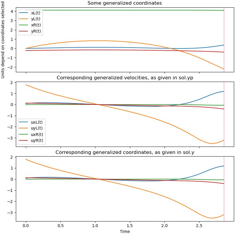
This marks, where solve_dae aborted. Used to plot the dotted red vertical line.
end_sol = sol.t[-1]
Plot some generalized coordinates.
bezeichnung = [str(i) for i in q_ind + u_ind]
fig, ax = plt.subplots(3, 1, figsize=(8, 8), sharex=True, layout='constrained')
for i in (1, 2, 10, 11):
ax[0].plot(sol.t, sol.y[i], label=bezeichnung[i])
ax[1].plot(sol.t, sol.yp[i], label=bezeichnung[i + 14])
ax[2].plot(sol.t, sol.y[i + 14], label=bezeichnung[i + 14])
for i in range(3):
ax[i].axvline(x=end_sol, color='r', linestyle='--', lw=0.5)
ax[0].set_title('Some generalized coordinates')
ax[2].set_title('Corresponding generalized coordinates, as given in sol.y')
ax[1].set_title('Corresponding generalized velocities, as given in sol.yp')
ax[-1].set_xlabel('Time')
ax[0].set_ylabel('Units depend on coordinates selected')
ax[0].legend(loc='best')
_ = ax[1].legend(loc='best')
Plot some results.
def plot_simulation_results(times, valuesy, valuesyp):
colors1 = plt.cm.tab10(np.linspace(0, 1, 9))
fig, ax = plt.subplots(7, 1, figsize=(8, 23), layout='constrained',
sharex=True)
kin_np_v = np.array([kin_lam(*valuesy[0: 28, i], *pL_vals)
for i in range(valuesy.shape[1])])
kin_np_vp = np.array([kin_lam(*valuesy[0: 14, i], *valuesyp[0: 14, i],
*pL_vals)
for i in range(valuesy.shape[1])])
pot_np = np.array([pot_lam(*valuesy[0: 28, i], *pL_vals)
for i in range(valuesy.shape[1])])
total_np_v = kin_np_v + pot_np
total_np_vp = kin_np_vp + pot_np
for i in range(37, 41):
ax[0].plot(times, valuesyp[i, :],
label=rf'$\dot{{\kappa_{{nh}}}}_{{{i-37}}}$',
color=colors1[i-37])
ax[0].set_title(r'$\dot{\kappa}_{nh}$ Values', fontsize=13)
ax[0].legend(fontsize=11, loc='upper left')
for i in range(28, 37):
ax[1].plot(times, valuesyp[i, :],
label=rf'$\dot{{\kappa}}_{{{i-28}}}$',
color=colors1[i-28])
ax[1].set_title(r'$\dot{\kappa}$ Values', fontsize=13)
ax[1].legend(fontsize=11, loc='upper left')
ax[2].plot(times, kin_np_v, label='Kinetic Energy')
ax[2].plot(times, pot_np, label='Potential Energy')
ax[2].plot(times, total_np_v, label='Total Energy')
ax[2].set_xlabel('Time [s]')
ax[2].set_ylabel('Energy')
ax[2].set_title('Energy', fontsize=13)
ax[2].legend(fontsize=11)
for i in range(9):
ax[3].plot(times, [hol_plot_lam(*valuesy[0:28, j], *pL_vals)[i]
for j in range(valuesy.shape[1])],
label='hol constr.' + str(i))
ax[3].set_ylabel('Constraint Values')
ax[3].set_title('Holonomic Constraints', fontsize=13)
ax[3].legend(fontsize=11)
for i in range(4):
ax[4].plot(times, [nonhol_plot_lam(*valuesy[0:28, j], *pL_vals)[i]
for j in range(valuesy.shape[1])],
label='nonhol constr.' + str(i))
ax[4].set_ylabel('Constraint Values')
ax[4].set_title('Nonholonomic Constraints', fontsize=13)
ax[4].legend(fontsize=11)
ax[5].plot(t_list[1:], A_vel_list, label='A_vel')
ax[5].plot(t_list[1:], MM_free_list, label='MM_free')
ax[5].legend(fontsize=11)
ax[5].set_yscale('log')
ax[5].set_title('Condition Number of A_vel and MM_free', fontsize=13)
ax[6].plot(t_list[1:], hol_grad_list, label='Holonomic Gradient')
ax[6].plot(t_list[1:], nonhol_grad_list, label='Nonholonomic Gradient')
ax[6].legend(fontsize=11)
ax[6].set_title('Condition Number of Holonomic and Nonholonomic Gradients',
fontsize=13)
if reibung1 == 0.0:
delta_energy_v = ((np.max(total_np_v) - np.min(total_np_v)) /
np.max(total_np_v))
delta_energy_vp = ((np.max(total_np_vp) - np.min(total_np_vp)) /
np.max(total_np_vp))
print("Deviation of total energy from being constant: "
f"{delta_energy_v:.3e} with speeds taken from y"
f" obervation time up to {times[-1]:.3f} sec")
print("Deviation of total energy from being constant: "
f"{delta_energy_vp:.3e} with speeds taken from yp"
f" obervation time up to {times[-1]:.3f} sec")
for i in range(7):
ax[i].axvline(x=end_sol, color='r', linestyle='--', lw=0.5)
plot_simulation_results(sol.t, sol.y, sol.yp)
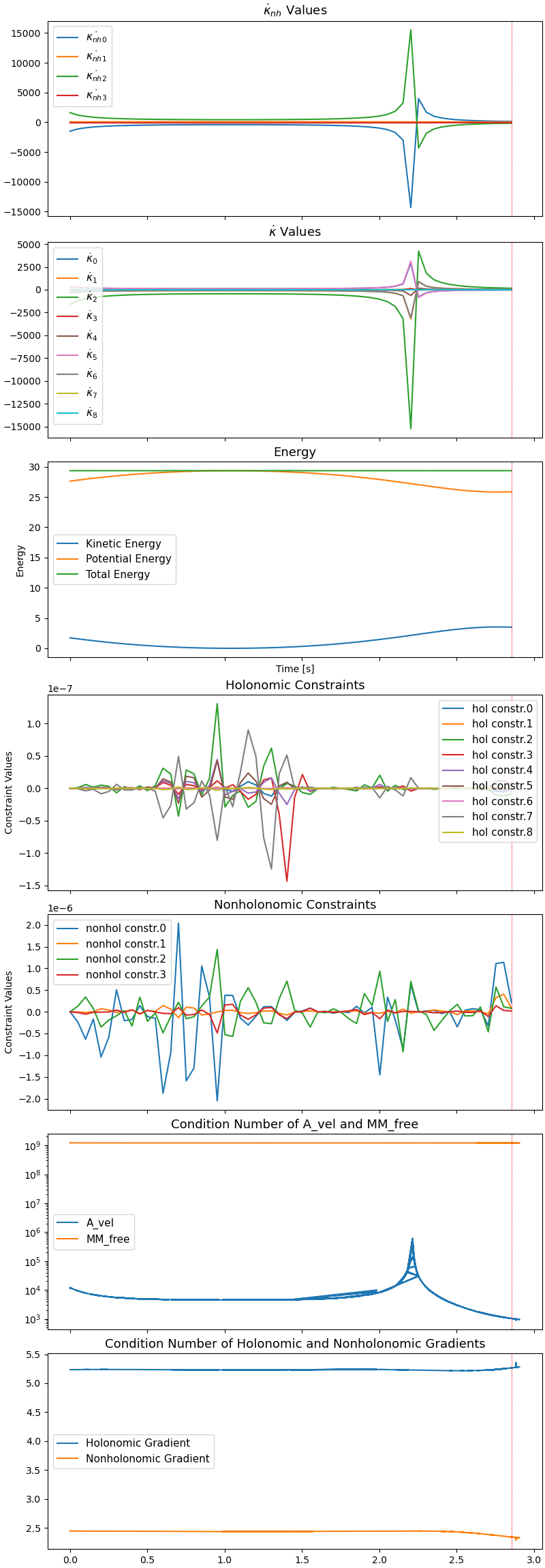
Deviation of total energy from being constant: 9.358e-05 with speeds taken from y obervation time up to 2.856 sec
Deviation of total energy from being constant: 1.349e-03 with speeds taken from yp obervation time up to 2.856 sec
Integrate using IDA.
A_vel_list = []
MM_free_list = []
hol_grad_list = []
nonhol_grad_list = []
t_list = [0.0]
result = np.empty(50)
def residual(t, v, vp, result):
A_vel_list.append(np.linalg.cond(A_vel_lam(*v[0: 15], *pL_vals)))
MM_free_list.append(np.linalg.cond(MM_free_lam(*v[0: 28], *pL_vals)))
hol_grad_list.append(np.linalg.cond(hol_grad_lam(*v[0: 28], *pL_vals)))
nonhol_grad_list.append(np.linalg.cond(nonhol_grad_lam(*v[0: 28],
*pL_vals)))
t_list.append(t)
result[0: 14] = F0_lam(*v, *vp, *pL_vals).squeeze()
result[14: 28] = F1_lam(*v, *vp, *pL_vals).squeeze()
result[28: 37] = F2_lam(*v, *vp, *pL_vals).squeeze()
result[37: 46] = F3_lam(*v, *vp, *pL_vals).squeeze()
result[46: 50] = F4_lam(*v, *vp, *pL_vals).squeeze()
f0 = residual(0.0, v001, vp001, result)
print("norm of residual with the initial values, "
f"{np.linalg.norm(result):.3e}")
solver = dae(
"ida",
residual,
old_api=False,
rtol=rtol,
atol=atol_dae,
)
tout = np.linspace(0.0, tf, schritte)
solution_i = solver.solve(tout, v001, vp001)
print(solution_i.message)
t_arr = solution_i.values.t
y_arr = solution_i.values.y
yp_arr = solution_i.values.ydot
print(t_arr[-1])
norm of residual with the initial values, 1.588e-09
No module named 'scikits_odes_daepack'
No module named 'scikits_odes_daepack'
Successful function return.
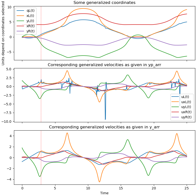
25.0
Plot some generalized coordinates.
bezeichnung = [str(i) for i in q_ind + u_ind]
fig, ax = plt.subplots(3, 1, figsize=(8, 8), sharex=True, layout='constrained')
for i in (0, 1, 2, 10, 11):
ax[0].plot(t_arr, y_arr.T[i], label=bezeichnung[i])
ax[1].plot(t_arr, yp_arr.T[i], label=bezeichnung[i + 14])
ax[2].plot(t_arr, y_arr.T[14 + i], label=bezeichnung[i + 14])
for i in range(3):
ax[i].axvline(x=end_sol, color='r', linestyle='--', lw=0.5)
ax[0].set_title('Some generalized coordinates')
ax[1].set_title('Corresponding generalized velocities as given in yp_arr')
ax[2].set_title('Corresponding generalized velocities as given in y_arr')
ax[-1].set_xlabel('Time')
ax[0].set_ylabel('Units depend on coordinates selected')
ax[0].legend(loc='best')
_ = ax[1].legend(loc='best')
Plot some results.
plot_simulation_results(t_arr.T, y_arr.T, yp_arr.T)
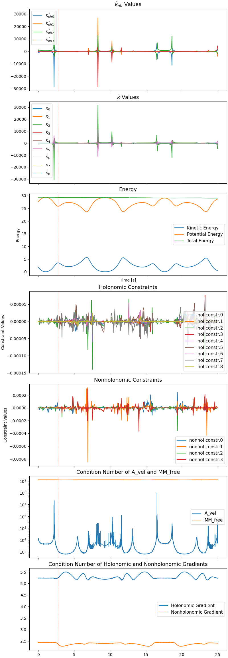
Deviation of total energy from being constant: 1.040e-02 with speeds taken from y obervation time up to 25.000 sec
Deviation of total energy from being constant: 7.706e-01 with speeds taken from yp obervation time up to 25.000 sec
Animation
fps = 7
times = t_arr
resultat = y_arr
time_arr = times
state_sol = interp1d(time_arr, resultat, kind='cubic', axis=0)
coordinates = DmcL.pos_from(O).to_matrix(N)
for point in (DmcR, PL, PR):
coordinates = coordinates.row_join(point.pos_from(O).to_matrix(N))
coords_lam = sm.lambdify(qLL + pLL, coordinates, cse=True)
max_x = np.max(resultat[:, 1]) + lax1 + max(rL1, rR1)
max_y = np.max(resultat[:, 2]) + max(rL1, rR1)
min_x = np.min(resultat[:, 1]) - lax1 - max(rL1, rR1)
min_y = np.min(resultat[:, 2]) - max(rL1, rR1)
gesamt_plot_lam = sm.lambdify([x_h, y_h, amplitude, frequenz],
gesamt_plot(x_h, y_h, amplitude, frequenz),
cse=True)
max_radius = 2.0 * max(rL1, rR1)
xx = np.linspace(min_x-max_radius, max_x+max_radius, 100)
yy = np.linspace(min_y-max_radius, max_y+max_radius, 100)
XX, YY = np.meshgrid(xx, yy)
ZZ = gesamt_plot_lam(XX, YY, amplitude1, frequenz1)
fig, ax = plt.subplots(figsize=(8, 8))
ax.set_xlim(min_x, max_x)
ax.set_ylim(min_y, max_y)
ax.set_aspect('equal')
ax.set_xlabel('x', fontsize=15)
ax.set_ylabel('y', fontsize=15)
cf = ax.contourf(XX, YY, ZZ, levels=50, cmap='viridis')
fig.colorbar(cf, label='z value [m]', shrink=0.5)
line1, = ax.plot([], [], lw=1, marker='o', markersize=0, color='red')
line4 = ax.scatter([], [], color='black', s=20)
line5 = ax.scatter([], [], color='black', s=20)
# ellipses defined in local frame AX
winkel_q2 = state_sol(0)[13]
ellipseL = Ellipse((0, 0), width=2.0*rL1*np.sin(winkel_q2),
height=2.0*rL1,
fill=True, lw=2, color='red', alpha=0.5)
ax.add_patch(ellipseL)
ellipseR = Ellipse((0, 0), width=2.0*rR1*np.sin(winkel_q2),
height=2.0*rR1,
fill=True, lw=2, color='magenta', alpha=0.5)
ax.add_patch(ellipseR)
def update(t):
message = (f'Running time {t:.2f} sec \n'
f'The left wheel is red with radius {rL1}, the '
f'right wheel is magenta \n with radius {rR1},'
f' The black dots are the particles attached \n to the wheels')
ax.set_title(message, fontsize=11)
coords = coords_lam(*state_sol(t)[0: 28], *pL_vals)
line1.set_data([coords[0, 0], coords[0, 1]], [coords[1, 0],
coords[1, 1]])
line4.set_offsets([coords[0, 2], coords[1, 2]])
line5.set_offsets([coords[0, 3], coords[1, 3]])
# transform from AX → inertial frame
theta = state_sol(t)[3]
X = coords[0, 0]
Y = coords[1, 0]
transform = Affine2D().rotate(theta).translate(X, Y) + ax.transData
ellipseL.set_width(2.0*rL1*np.sin(-state_sol(t)[13]))
ellipseL.set_transform(transform)
X = coords[0, 1]
Y = coords[1, 1]
transform = Affine2D().rotate(theta).translate(X, Y) + ax.transData
ellipseR.set_width(2.0*rR1*np.sin(-state_sol(t)[13]))
ellipseR.set_transform(transform)
return line1, line4, line5, ellipseL, ellipseR
# Create the animation
animation = FuncAnimation(fig, update,
frames=np.concatenate([np.arange(
0, times[-1], 1.0/fps), [times[-1]]]),
interval=1000/fps, blit=False)
plt.show()