Brachistochrone with Obstruction

Objective

• Show how to solve a variational problem using opty with variable time interval.

Introduction

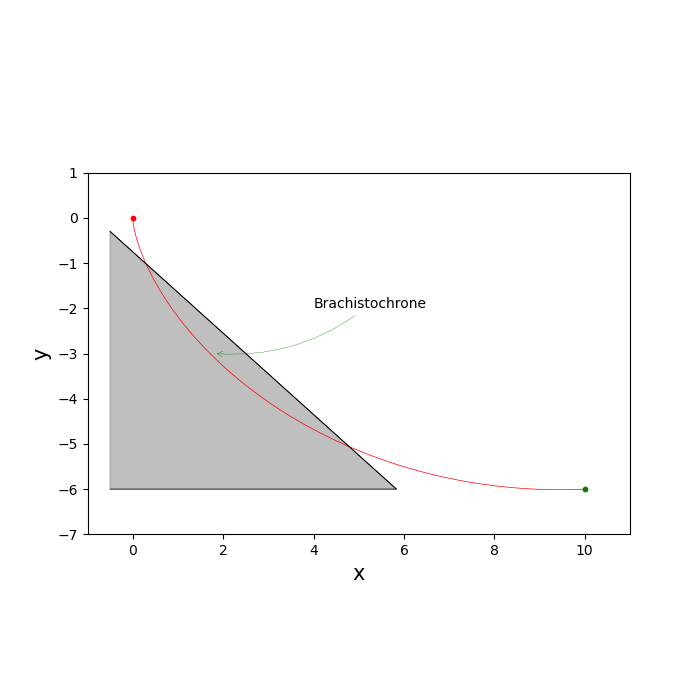
A particle is to slide without friction under the constant force of gravity on a curve from A to B in the shortest time. B must not be directly under A (else the problem is trivial). The solution curve is called the Brachistochrone which is a cycloid. On part of the path, there is a line that the particle must not cross.

Explanation of the Approach Taken

Let the curve be called \(b(x)\). If the particle is at \((x(t) , b(x(t))\) then it cannot have a speed component normal to the tangent of the curve at this point. This fact is used to set up the equations of motion. Without loss of generality the starting point is (0, 0). The interfering line is a holonomic inequality constraint. The inequality is enforced by bounding the relevant algebraic equation in the equations of motion.

The simulation is similar, but not identical to the example in John T. Betts, Practical Methods for Optimal Control Using Nonlinear Programming, 3rd Edition, section 4.16.2

Notes

The curve is parameterized by time and a nonholonomic constraint is introduced to ensure the motion is always tangent to the curve. The nonholonomic constraint is similar to the constraint present in the Chaplygin Sleigh.

States

• \(x\): x-coordinate of the particle

• \(y\): y-coordinate of the particle, opposite in sign to the gravitational force

• \(u_x\): x-component of the velocity of the particle

• \(u_y\): y-component of the velocity of the particle

Inputs

• \(\beta\): angle of the tangent of the curve with the horizontal

Known Parameters

• \(m\): mass of the particle

• \(g\): acceleration due to gravity

• \(b_1\): x coordinate of the final point

• \(b_2\): y coordinate of the final point

• \(h_{\textrm{shift}}\): shift of the curve in the -y direction

• \(\text{steepness}\): slope of the interfering line

Free Parameters

• \(h\): time interval

import numpy as np
import sympy as sm
import sympy.physics.mechanics as me
import matplotlib.pyplot as plt
from opty import Problem
from scipy.optimize import root
from scipy.interpolate import CubicSpline
from matplotlib.animation import FuncAnimation
from opty.utils import MathJaxRepr


import time

Equations of Motion

The equations of motion represent a particle \(P\) of mass \(m\) moving in a uniform gravitational field. The point moves on a surface that applies a normal force to it and the angle of the surface relative to the horizontal is \(\beta(t)\). A nonholonomic constraint to ensure the particle’s velocity only has a component tangent to the surface is added to the equations of motion. In addition, a holonomic inequality is added, making it a set of differential algebraic equations.

N, A = me.ReferenceFrame('N'), me.ReferenceFrame('A')
O, P = sm.symbols('O P', cls=me.Point)
O.set_vel(N, 0)
t = me.dynamicsymbols._t

m, g, h_shift, steepness = sm.symbols('m, g, h_shift, steepness')
x, y, ux, uy = me.dynamicsymbols('x y u_x u_y')
beta = me.dynamicsymbols('beta')

state_symbols = (x, y, ux, uy)

A.orient_axis(N, beta, N.z)

P.set_pos(O, x*N.x + y*N.y)
P.set_vel(N, ux*N.x + uy*N.y)

speed_constr = sm.Matrix([P.vel(N).dot(A.y)])

kd = sm.Matrix([ux - x.diff(t), uy - y.diff(t)])

bodies = [me.Particle('body', P, m)]
forces = [(P, -m*g*N.y)]

kane = me.KanesMethod(
    N,
    q_ind=[x, y],
    u_ind=[ux],
    u_dependent=[uy],
    kd_eqs=kd,
    velocity_constraints=speed_constr,
)
fr, frstar = kane.kanes_equations(bodies, loads=forces)

eom = kd.col_join(fr + frstar)
eom = eom.col_join(speed_constr)
eom = eom.col_join(sm.Matrix([(-y - steepness*x - h_shift)]))
MathJaxRepr(eom)

$$\left[\begin{matrix}u_{x} - \dot{x}\\u_{y} - \dot{y}\\- \frac{g m \sin{\left(\beta \right)}}{\cos{\left(\beta \right)}} - \frac{m \sin{\left(\beta \right)} \dot{u}_{y}}{\cos{\left(\beta \right)}} - m \dot{u}_{x}\\- u_{x} \sin{\left(\beta \right)} + u_{y} \cos{\left(\beta \right)}\\- h_{shift} - steepness x - y\end{matrix}\right]$$

Set up the Optimization Problem and Solve It

The goal is to minimize the time to reach the second point. So make the time interval a variable \(h\).

h = sm.symbols('h')
num_nodes = 201
t0, tf = 0*h, h*(num_nodes - 1)


def obj(free):
    return free[-1]


def obj_grad(free):
    grad = np.zeros_like(free)
    grad[-1] = 1.0
    return grad

Set up the constraints and bounds, objective function and its gradient for the problem. (b1, b2) is the final point and (0, 0) is the starting point is (0/0).

b1 = 10.0
b2 = -6.0

par_map = {
        m: 1.0, g: 9.81,
        h_shift: 0.75,
        steepness: 0.9,
}


instance_constraint = (
    x.func(t0),
    y.func(t0),
    ux.func(t0),
    uy.func(t0),
    x.func(tf) - b1,
    y.func(tf) - b2,
)

bounds = {
    h: (0.0, 1.0),
    beta: (-np.pi/2 + 1.e-5, 0.0),
}
eom_bounds = {4: (-np.inf, 0.0)}

Set Up the Problem.

prob = Problem(
        obj,
        obj_grad,
        eom,
        state_symbols,
        num_nodes,
        h,
        time_symbol=t,
        known_parameter_map=par_map,
        instance_constraints=instance_constraint,
        bounds=bounds,
        eom_bounds=eom_bounds,
    )

Solve the problem.

zeit = time.time()
np.random.seed(123)
initial_guess = np.random.randn(prob.num_free)*0.1
prob.add_option('max_iter', 55000)
solution, info = prob.solve(initial_guess)
print(info['status_msg'])
prob.plot_objective_value()

print(('time taken to solve the problem: '
       f'{time.time() - zeit:.2f} sec'))

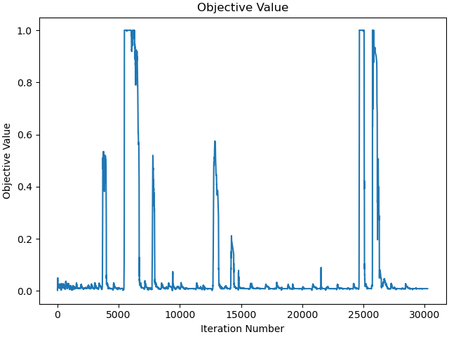
b'Algorithm terminated successfully at a locally optimal point, satisfying the convergence tolerances (can be specified by options).'
time taken to solve the problem: 213.85 sec

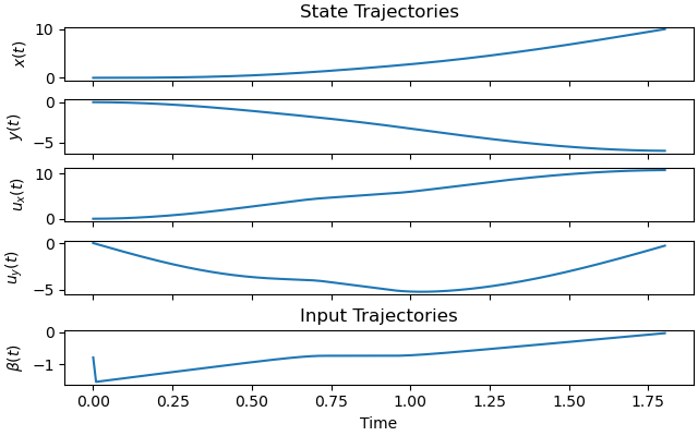
State and input trajectories:

_ = prob.plot_trajectories(solution)

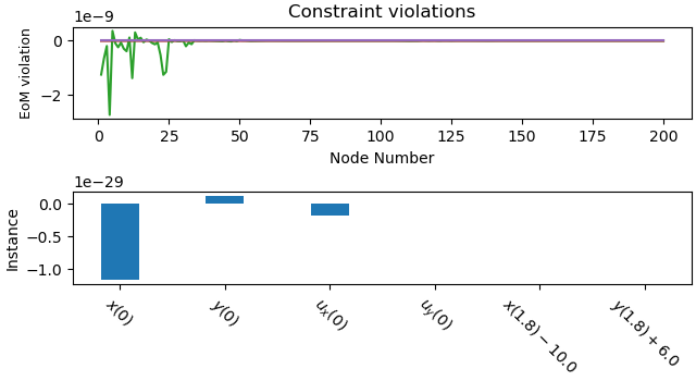
Constraint violations:

_ = prob.plot_constraint_violations(solution)

Animate the Solution

fps = 35

Calculate the Brachistochrone from (0, 0) to (b1, b2). It is very sensitive to the initial guess.

def func(x0):
    """Gives the Brachistochrome equation for the starting point at (0, 0) and
    the final point at (b1, b2)"""
    r, theta = x0[0], x0[1]
    return [r*theta - r*np.sin(theta) - b1, r*(1.0 - np.cos(theta)) - b2]


x0 = [1.0, 1.0]
resultat = root(func, x0)

times = np.linspace(0.0, resultat.x[1], num_nodes)
xx = resultat.x[0]*times - resultat.x[0]*np.sin(times)
yy = resultat.x[0]*(1.0 - np.cos(times))

Set up the plot.

state_vals, input_vals, _, h_val = prob.parse_free(solution)
t_arr = np.linspace(t0, num_nodes*solution[-1], num_nodes)
state_sol = CubicSpline(t_arr, state_vals.T)
input_sol = CubicSpline(t_arr, input_vals.T)

xmin = -1.0
xmax = b1 + 1.0
ymin = b2 - 1.0
ymax = 1.0

arrow_head = me.Point('arrow_head')
arrow_head.set_pos(P, ux*N.x + uy*N.y)

coordinates = P.pos_from(O).to_matrix(N)
coordinates = coordinates.row_join(arrow_head.pos_from(O).to_matrix(N))

coords_lam = sm.lambdify(list(state_symbols) + [beta] + list(par_map.keys()),
                         coordinates, cse=True)

def init_plot():
    fig, ax = plt.subplots(figsize=(7, 7))
    ax.set_xlim(xmin, xmax)
    ax.set_ylim(ymin, ymax)
    ax.set_aspect('equal')
    ax.set_xlabel('x', fontsize=15)
    ax.set_ylabel('y', fontsize=15)

    # Plot the Brachistochrone analytical solution.
    ax.plot(xx, yy, color='red', lw=0.5)
    ax.scatter([0], [0], color='red', s=10)
    ax.scatter([b1], [b2], color='green', s=10)


    # plot the restrictive line
    start_x = -0.5
    ax.plot([start_x, -(b2 + par_map[h_shift])/par_map[steepness]],
            [-par_map[steepness]*start_x-par_map[h_shift], b2],
            color='black', lw=0.5)

    # shade the 'forbidden triangle
    triangle_x = [start_x, -(b2 + par_map[h_shift])/par_map[steepness],
                 start_x]
    triangle_y = [-par_map[steepness]*start_x-par_map[h_shift], b2, b2]
    ax.fill(triangle_x, triangle_y, color='gray', alpha=0.5)
    ax.plot(triangle_x, triangle_y, color='black', lw=0.5)

    ax.annotate('Brachistochrone', xy=(1.8, -3),
                arrowprops=dict(arrowstyle='->',
                        connectionstyle='arc3, rad=-.2', color='green',
                        lw=0.25),
                xytext=(4.0, -2.0), fontsize=10)

    # Set up the point and the speed arrow.
    punkt = ax.scatter([], [], color='red', s=50)
    # Draw the speed vector.
    pfeil = ax.quiver([], [], [], [], color='green', scale=25, width=0.004)

    return fig, ax, punkt, pfeil

Function to update the plot for each animation frame

fig, ax, punkt, pfeil = init_plot()


def update(t):
    message = (f'Running time {t:.2f} sec \n'
               f'The green arrow is the speed \n'
               f'Slow motion video.')
    ax.set_title(message, fontsize=12)

    coords = coords_lam(*state_sol(t), input_sol(t), *par_map.values())
    punkt.set_offsets([coords[0, 0], coords[1, 0]])

    pfeil.set_offsets([coords[0, 0], coords[1, 0]])
    pfeil.set_UVC(coords[0, 1] - coords[0, 0], coords[1, 1] - coords[1, 0])

Create the animation.

fig, ax, punkt, pfeil = init_plot()
animation = FuncAnimation(
    fig,
    update,
    frames=np.arange(t0, (num_nodes + 2)*h_val, 1/fps),
    interval=3000/fps,
)

plt.show()

Once Loop Reflect