Note

Go to the end to download the full example code.

Glocker and Leine Problem¶

Objective¶

Show how to uses solve_dae and Sundials’ IDA to integrate a system with holonomic and non-holonomic constraints, using the Hiller/Anatharaman formulation.

Description¶

A disc of mass $m$ and radius $r$ rolls without slipping on the horizontal X/Y plane. Gravity points in the negative Z direction. There is no friction present. More can likely be found here: https://www.sciencedirect.com/science/article/pii/S0020740317301550

Notes¶

The Hiller/Anatharaman formulation used to integrate the system with holonomic and non-holonomic constraints was given by Jonas Breuling (private communication).
solve_dae (presently) allows the methods ‘BDF’ and ‘Radau’. Tests here indicate that ‘BDF’ is more stable than ‘Radau’ for this problem.
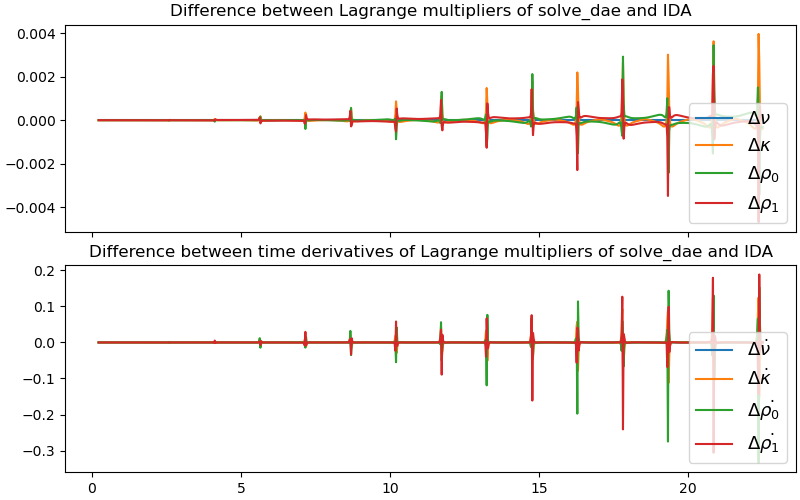
Test here also indicate that solve_dae is more accurate than Sundials’ IDA for this problem, but it is less stable in the sense that it aborts earlier.
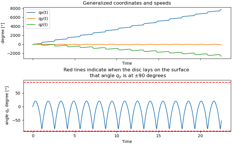
There being no friction, the total energy should be constant. If this constancy is a measure of overall accuracy (I do not know if this is so), then solve_ivp is the most accurate.
It seems, that the disc never lays flat on the surface, but in the last minute so to speak it uprights itself again.

States

$q_x, q_y, q_z$ are the angular coordinates of the disc.
$x, y, z$ are the Cartesian coordinates of the center of mass of the disc.
$u_{q_x}, u_{q_y}, u_{q_z}$ are the angular speeds of the disc.
$u_x, u_y, u_z$ are the Cartesian speeds of the center of mass of the disc.
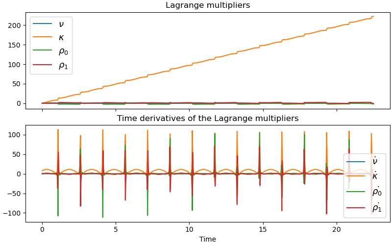
$\nu, \kappa, \rho$ are the Lagrange multipliers.
$\dot{\nu}, \dot{\kappa}, \dot{\rho}$ are the time derivatives of the Lagrange multipliers.
$v$ is the vector of all states needed for solve_dae and Sundials’ IDA.
$v_p = \dot{v}$ is the time derivative of $v$.

Parameters

$m$ is the mass of the disc.
$g$ is the gravitational acceleration.
$r$ is the radius of the disc.

import sympy as sm
import sympy.physics.mechanics as me
import numpy as np
import matplotlib.pyplot as plt
from scipy.integrate import solve_ivp
from scipy.interpolate import interp1d
from solve_dae.integrate import solve_dae, consistent_initial_conditions
from scikits.odes import dae
from matplotlib.animation import FuncAnimation

Kane’s Equations of Motion.¶

N, A, AX = sm.symbols('N A AX', cls=me.ReferenceFrame)
O, Dmc, CP = sm.symbols('O Dmc CP', cls=me.Point)
t = me.dynamicsymbols._t
O.set_vel(N, 0)

Coordinates of the center of the disc.

x, y, z, ux, uy, uz = me.dynamicsymbols('x y z ux uy uz')

Angular coordinates of the disc.

qx, qy, qz, uqx, uqy, uqz = me.dynamicsymbols('qx qy qz uqx uqy uqz')

Virtual speeds and noncontributing forces.

auxx, auxy, auxz, fx, fy, fz = me.dynamicsymbols('auxx auxy auxz fx fy fz')
all_zero = dict.fromkeys([auxx, auxy, auxz,
                          auxx.diff(t), auxy.diff(t), auxz.diff(t),
                          fx, fy, fz], 0)

Locate the center of mass of the disc and its velocity in the inertial frame.

Dmc.set_pos(O, x*N.x + y*N.y + z*N.z)
Dmc.set_vel(N, ux*N.x + uy*N.y + uz*N.z)

Body fixed frame of the disc.

A.orient_body_fixed(N, [qz, qy, qx], 'ZYX')

Axle of the disc. The disc rotates around AX.x.

AX.orient_body_fixed(N, [qz, qy, 0], 'ZYX')

Some constants.

m, g, r = sm.symbols('m g r')

Define the contact point of the disc with the plane.

CP.set_pos(Dmc, -r*AX.z)
CP.set_vel(N, Dmc.vel(N) + A.ang_vel_in(N).cross(-r*AX.z))

Holonomic constraint: the contact point must remain on the plane z = 0.

hol_constr = sm.Matrix([CP.pos_from(O).dot(N.z)])

Non-holonomic constraints: the contact point must have zero velocity.

non_hol_constr = sm.Matrix([CP.vel(N).dot(N.x),
                            CP.vel(N).dot(N.y)
                            ])

Rigid Body.

iXX = 1/2 * m * r**2
iYY = 1/4 * m * r**2
iZZ = 1/4 * m * r**2
I_disc = me.inertia(A, iXX, iYY, iZZ)
disc = me.RigidBody('disc', Dmc, A, m, (I_disc, Dmc))
bodies = [disc]

Forces.

F_gravity = (Dmc, -m*g*N.z)
F_noncontrib = (CP, fx*N.x + fy*N.y + fz*N.z)
forces = [F_gravity, F_noncontrib]

Kinematic DEs.

kd = sm.Matrix([
    qx.diff(t) - uqx,
    qy.diff(t) - uqy,
    qz.diff(t) - uqz,
    x.diff(t) - ux,
    y.diff(t) - uy,
    z.diff(t) - uz,
])

Time differentiation of the holonomic constraint and appending the non-holonomic constraints gives the velocity constraints, needed for Kane’s method. The virtual speeds of the contact point must be added here.

speed_constr = hol_constr.diff(t).col_join(non_hol_constr)
speed_constr = speed_constr + sm.Matrix([auxz, auxx, auxy])

q_ind = [qx, qy, qz, x, y]
q_dep = [z]
u_ind = [uqx, uqy, uqz]
u_dep = [ux, uy, uz]

aux = [auxx, auxy, auxz]

kane = me.KanesMethod(
    N,
    q_ind,
    u_ind,
    q_dependent=q_dep,
    u_dependent=u_dep,
    u_auxiliary=aux,
    kd_eqs=kd,
    configuration_constraints=hol_constr,
    velocity_constraints=speed_constr,
    )

fr, frstar = kane.kanes_equations(bodies, forces)
MM = kane.mass_matrix_full
force = kane.forcing_full
force = me.msubs(force, all_zero)
MM = me.msubs(MM, all_zero)
noncontrib_forces = kane.auxiliary_eqs


print(f"the mass matrix contains {sm.count_ops(MM):,} operations")
print(f"the forcing vector contains {sm.count_ops(force):,} operations")

the mass matrix contains 1,881 operations
the forcing vector contains 6,113 operations

Prepare for the reaction forces. The accelerations must be replaced with placeholders until available.

pL = [m, g, r]
qL = q_ind + q_dep + u_ind + u_dep

rhs = sm.symbols('rhs:12')
rhs_dict = {i.diff(t): j for i, j in zip(q_ind + q_dep + u_ind + u_dep, rhs)}
noncontrib_forces = me.msubs(noncontrib_forces, rhs_dict)
noncontrib_forces

Areact, breact = sm.linear_eq_to_matrix(noncontrib_forces, (fx, fy, fz))
react_forces = Areact.LUsolve(breact)
react_forces
react_lam = sm.lambdify(q_ind + q_dep + u_ind + u_dep + list(rhs) + pL,
                        react_forces, cse=True)

Solve for the dependent speeds ux, uy, uz.

kin_dict = {i.diff(t): j for i, j in zip(q_ind + q_dep, u_ind + u_dep)}

speed_constr = me.msubs(speed_constr, kin_dict, all_zero)
A_nh, b_nh = sm.linear_eq_to_matrix(speed_constr, (ux, uy, uz))
res_dep_speed = A_nh.LUsolve(b_nh)

# Compilation.
pL = [m, g, r]
qL = q_ind + q_dep + u_ind + u_dep

MM_lam = sm.lambdify(qL + pL, MM, cse=True)
force_lam = sm.lambdify(qL + pL, force, cse=True)
res_dep_speed_lam = sm.lambdify(q_ind + q_dep + u_ind + pL, res_dep_speed,
                                cse=True)

Energy, constraints.

kin_energy = me.msubs(disc.kinetic_energy(N), kin_dict, all_zero)
pot_energy = m * g * Dmc.pos_from(O).dot(N.z)

kin_lam = sm.lambdify(qL + pL, kin_energy, cse=True)
pot_lam = sm.lambdify(qL + pL, pot_energy, cse=True)

hol_lam = sm.lambdify(qL + pL, hol_constr, cse=True)
non_hol_constr = me.msubs(non_hol_constr, kin_dict)
non_hol_lam = sm.lambdify(qL + pL, non_hol_constr, cse=True)

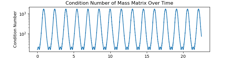
Get the condition number of the unconstrained mass matrix, with the values of the constrained solution. Only information, not needed.

q_dae_ind = q_ind + q_dep
u_dae_ind = u_ind + u_dep
kane_unconstrained = me.KanesMethod(
    N,
    q_dae_ind,
    u_dae_ind,
    kd_eqs=kd
)
fr, frstar = kane_unconstrained.kanes_equations(bodies, forces)
M_unconstrained = me.msubs(kane_unconstrained.mass_matrix, all_zero)
F_unconstrained = me.msubs(kane_unconstrained.forcing, all_zero)

M_unconstrained_lam = sm.lambdify(q_dae_ind + u_dae_ind + pL, M_unconstrained)

MM_test = kane_unconstrained.mass_matrix_full
MM_test_lam = sm.lambdify(q_dae_ind + u_dae_ind + pL, MM_test)

force_test = kane_unconstrained.forcing_full
force_test_lam = sm.lambdify(q_dae_ind + u_dae_ind + pL, force_test)

Use solve_ivp for numerical integration.

cond_list = []


def gradient(t, y, args):
    cond_list.append(np.linalg.cond(M_unconstrained_lam(*y, *args)))
    sol = np.linalg.solve(MM_lam(*y, *args), force_lam(*y, *args))
    return sol.squeeze()

Parameter Values.

m1 = 1
g1 = 9.81
r1 = 0.5
pL_vals = [m1, g1, r1]

Initial conditions.

x1 = 0
y1 = 0

qx1 = 0.0
qy1 = 0.0
qz1 = 0.0
uqx1 = 2.0
uqy1 = 2.0
uqz1 = 2.0

Get z1 directly from the holonomic constraint. (For a more difficult problem, this would have to be solved numerically.)

z1 = r1 * np.cos(qy1)

Solve for the dependent speeds using the initial conditions.

ux1, uy1, uz1 = res_dep_speed_lam(qx1, qy1, qz1, x1, y1, z1, uqx1,
                                  uqy1, uqz1, *pL_vals)
ux1 = ux1[0]
uy1 = uy1[0]
uz1 = uz1[0]

Starting vector.

y0 = [qx1, qy1, qz1, x1, y1, z1, uqx1, uqy1, uqz1, ux1, uy1, uz1]

Integration with solve_ivp starts.

t0, tf = 0.0, 22.5
schritte = 1000
t_eval = np.linspace(t0, tf, schritte)
atol = 1e-9
rtol = 1e-8
method = 'Radau'

resultat1 = solve_ivp(
    gradient,
    (t0, tf), y0,
    t_eval=t_eval,
    args=(pL_vals,),
    method=method,
    atol=atol,
    rtol=rtol,
    )

print(resultat1.message)

The solver successfully reached the end of the integration interval.

Plot the condition number of the mass matrix of the unconstrained system, evaluated at the solution of the system with speed constraints.

fig, ax = plt.subplots(figsize=(8, 2))
ax.plot(np.linspace(t0, tf, len(cond_list)), cond_list)
ax.set_yscale('log')
ax.set_xlabel('Time')
ax.set_ylabel('Condition Number')
_ = ax.set_title('Condition Number of Mass Matrix Over Time')

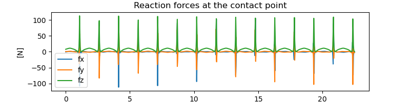
Condition Number of Mass Matrix Over Time

Calculate and plot the reaction forces at the contact points.

fx_np = np.empty(schritte)
fy_np = np.empty(schritte)
fz_np = np.empty(schritte)
for i in range(schritte):
    RHS = np.linalg.solve(
        MM_lam(*resultat1.y[:, i], *pL_vals),
        force_lam(*resultat1.y[:, i], *pL_vals)).squeeze()
    fx_np[i] = react_lam(*resultat1.y[:, i], *RHS, *pL_vals)[0].squeeze()
    fy_np[i] = react_lam(*resultat1.y[:, i], *RHS, *pL_vals)[1].squeeze()
    fz_np[i] = react_lam(*resultat1.y[:, i], *RHS, *pL_vals)[2].squeeze()

fig, ax = plt.subplots(figsize=(8, 2))
ax.plot(resultat1.t, fx_np, label='fx')
ax.plot(resultat1.t, fy_np, label='fy')
ax.plot(resultat1.t, fz_np, label='fz')
ax.set_xlabel('time')
ax.set_ylabel('[N]')
ax.set_title('Reaction forces at the contact point')
_ = ax.legend()

Some generalized coordinates.

bezeichnung = [str(i) for i in q_ind + q_dep + u_ind + u_dep]
fig, ax = plt.subplots(2, 1, figsize=(8, 5), sharex=True, layout='constrained')
for i in (0, 1, 2):
    ax[0].plot(resultat1.t, np.rad2deg(resultat1.y[i]), label=bezeichnung[i])
ax[0].set_xlabel('Time')
ax[0].set_ylabel('degree [°]')
ax[0].set_title('Generalized coordinates and speeds')
ax[1].plot(resultat1.t, np.rad2deg(resultat1.y[1]))
ax[1].axhline(90, color='red', linestyle='--')
ax[1].axhline(-90, color='red', linestyle='--')

ax[1].set_xlabel('Time')
ax[1].set_ylabel('angle $q_y$ degree [°]')
ax[1].set_title(f'Red lines indicate when the disc lays on the surface \n '
                f'that angle $q_y$ is at ±90 degrees')

_ = ax[0].legend()

Generalized coordinates and speeds, Red lines indicate when the disc lays on the surface that angle $q_y$ is at ±90 degrees

Prepare for solve_dae and for IDA¶

Use the Hiller/Anatharaman formulation if holonomic and nonholinomic constraints a present (Jonas Breuling, private communication)

$M \dot{u} = h$ the equations of motion of the unconstrained system
$g_h(q, t) = 0 \in \\R^1$ the holonomic constraints
$g_{nh}(q, u, t) = \dfrac{\partial{{g_{nh}(q, u, t)}}}{\partial{u}} \cdot u + \dfrac{\partial{{g_{h}(q, u, t)}}}{\partial{t}} = 0 \in \\R^2$ the (linear) nonholonomic constraints
$\dot{q} = u$

$F_0 = \dot{q} - u - \left( \dfrac{\partial{{g_{h}(q, u, t)}}} {\partial{q}}\right)^T \cdot \dot{\nu} = 0 \in \\R^6$

$F_1 = M \dot{u} - h - \left(\dfrac{\partial{{g_{h}(q, u, t)}}} {\partial{q}} \right)^T \cdot \dot{\kappa} - \left(\dfrac{\partial{{g_{nh}(q, u, t)}}} {\partial{u}} \right)^T \cdot \dot{\rho } = 0 \in \\R^6$

$F_2 = \dfrac{d}{dt}g_h(q, t) = 0 \in \\R^1$

$F_3 = g_h(q, t) = 0 \in \\R^1$

$F_4 = g_{nh}(q, u, t) = 0 \in \\R^2$

Variables needed for solve_dae and for IDA.

v = me.dynamicsymbols('v:16')
vp = me.dynamicsymbols('vp:16')

Lagrange multipliers for the holonomic and non-holonomic constraints.

nu = me.dynamicsymbols('nu')
nudt = nu.diff(t)

kappa = me.dynamicsymbols('kappa')
kappadt = kappadt = kappa.diff(t)

rho = me.dynamicsymbols('rho:2')
rhodt = [i.diff(t) for i in rho]

Replacement dictionaries. Needed to replace the variables used to set up the equations of motion with the variables used in solve_dae and IDA.

v_dict = {i: j for i, j in zip(q_ind + q_dep + u_ind + u_dep +
                               [nu, kappa] + rho, v)}
vp_dict = {i.diff(t): j for i, j in zip(q_ind + q_dep + u_ind + u_dep +
                                        [nu, kappa] + rho, vp)}

First equation.

F0 = kd - hol_constr.jacobian(q_ind + q_dep).T * sm.Matrix([nudt])
F0 = me.msubs(F0, v_dict, all_zero)
F0 = me.msubs(F0, vp_dict)

Second equation.

Get the EOMs of the unconstrained system.

q_dae_ind = q_ind + q_dep
u_dae_ind = u_ind + u_dep
kane_unconstrained = me.KanesMethod(
    N,
    q_dae_ind,
    u_dae_ind,
    kd_eqs=kd
)
fr, frstar = kane_unconstrained.kanes_equations(bodies, forces)
M_unconstrained = kane_unconstrained.mass_matrix
F_unconstrained = kane_unconstrained.forcing

Now form F1.

F1 = (M_unconstrained * sm.Matrix([i.diff(t) for i in u_dae_ind]) -
      F_unconstrained -
      hol_constr.jacobian(q_ind + q_dep).T * sm.Matrix([kappadt]) -
      non_hol_constr.jacobian(u_ind + u_dep).T * sm.Matrix([i for i in rhodt]))

F1 = me.msubs(F1, v_dict, all_zero)
F1 = me.msubs(F1, vp_dict)

Third equation.

F2 = hol_constr.diff(t)
F2 = me.msubs(F2, kin_dict, all_zero)
F2 = me.msubs(F2, v_dict)
F2 = me.msubs(F2, vp_dict)

Forth equation

F3 = hol_constr
F3 = me.msubs(F3, v_dict, all_zero)
F3 = me.msubs(F3, vp_dict)

Fifth equation.

F4 = non_hol_constr
F4 = me.msubs(F4, v_dict, all_zero)
F4 = me.msubs(F4, vp_dict)

Complile the equations.

F0_lam = sm.lambdify(v + vp + pL, F0, cse=True)
F1_lam = sm.lambdify(v + vp + pL, F1, cse=True)
F2_lam = sm.lambdify(v + vp + pL, F2, cse=True)
F3_lam = sm.lambdify(v + vp + pL, F3, cse=True)
F4_lam = sm.lambdify(v + vp + pL, F4, cse=True)

Use solve_dae for numerical integration.

def F_solve_dae(t, v, vp):
    test = np.vstack((
        F0_lam(*v, *vp, *pL_vals),
        F1_lam(*v, *vp, *pL_vals),
        F2_lam(*v, *vp, *pL_vals),
        F3_lam(*v, *vp, *pL_vals),
        F4_lam(*v, *vp, *pL_vals)
    ))
    return test.squeeze()

Get consistent initial conditions.

v_start = y0 + [0] * 4
vp_start = np.zeros(len(v))

v01, vp01, f0 = consistent_initial_conditions(F_solve_dae, 0.0, v_start,
                                              vp_start)

The initial conditions must fulfill the equations. So || F(t0, v01, vp01) || = 0 is ideal.

print(f"||F(t0, v01, vp01)||: {np.linalg.norm(f0)} \n")

||F(t0, v01, vp01)||: 1.3042167484290357e-15

Integration starts.

method_dae = 'BDF'

sol = solve_dae(F_solve_dae, (t0, tf), v01, vp01,
                atol=atol,
                rtol=rtol,
                method=method_dae,
                t_eval=t_eval,
                )

success = sol.success
status = sol.status
message = sol.message
print(f"success: {success}")
print(f"status: {status}")
print(f"message: {message}")
print(f"nfev: {sol.nfev}")
print(f"njev: {sol.njev}")
print(f"nlu: {sol.nlu}")

C:\Users\Peter\anaconda3\envs\pst-notebooks-pydy\Lib\site-packages\scipy\integrate\_ivp\common.py:357: RuntimeWarning: overflow encountered in multiply
  h_new = (y[ind] + new_factor * y_scale[ind]) - y[ind]
C:\Users\Peter\anaconda3\envs\pst-notebooks-pydy\Lib\site-packages\scipy\integrate\_ivp\common.py:326: RuntimeWarning: overflow encountered in multiply
  h = (y + factor * y_scale) - y
C:\Users\Peter\anaconda3\envs\pst-notebooks-pydy\Lib\site-packages\scipy\integrate\_ivp\common.py:356: RuntimeWarning: overflow encountered in multiply
  new_factor = NUM_JAC_FACTOR_INCREASE * factor[ind]
C:\Users\Peter\anaconda3\envs\pst-notebooks-pydy\Lib\site-packages\scipy\integrate\_ivp\common.py:378: RuntimeWarning: overflow encountered in multiply
  factor[max_diff < NUM_JAC_DIFF_SMALL * scale] *= NUM_JAC_FACTOR_INCREASE
success: True
status: 0
message: The solver successfully reached the end of the integration interval.
nfev: 35321
njev: 1810
nlu: 2044

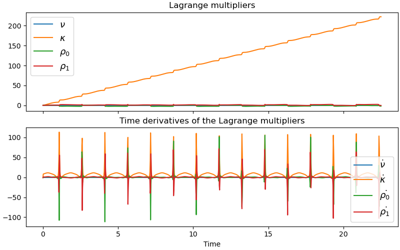
Plot Lagrange multipliers and their time derivatives.

bezeichnung = [r'$\nu$', r'$\kappa$', r'$\rho_0$', r'$\rho_1$']
bezeichnung_dot = [r'$\dot{\nu}$', r'$\dot{\kappa}$', r'$\dot{\rho_0}$',
                   r'$\dot{\rho_1}$']
fig, ax = plt.subplots(2, 1, figsize=(8, 5), layout='constrained', sharex=True)
for i in range(len(bezeichnung)):
    ax[0].plot(sol.t, sol.y[12 + i, :], label=bezeichnung[i])
    ax[1].plot(sol.t, sol.yp[12 + i, :], label=bezeichnung_dot[i])
ax[0]. set_title('Lagrange multipliers')
ax[1].set_title('Time derivatives of the Lagrange multipliers')
ax[-1].set_xlabel('Time')
ax[0].legend(fontsize=13)
_ = ax[1].legend(fontsize=13)

Lagrange multipliers, Time derivatives of the Lagrange multipliers

Use Sundials’ IDA for numerical integration.

def residual_HA(t, v, vp, result):
    result[0: 6] = F0_lam(*v, *vp, *pL_vals).squeeze()
    result[6: 12] = F1_lam(*v, *vp, *pL_vals).squeeze()
    result[12: 13] = F2_lam(*v, *vp, *pL_vals).squeeze()
    result[13: 14] = F3_lam(*v, *vp, *pL_vals).squeeze()
    result[14: 16] = F4_lam(*v, *vp, *pL_vals).squeeze()
    return 0


solver = dae(
    "ida",
    residual_HA,
    old_api=False,
    rtol=rtol,
    atol=atol,
)


t0, tf, n_out = 0.0, tf, schritte
tout = np.linspace(t0, tf, n_out)

solution_ida = solver.solve(tout, v01, vp01)
print(solution_ida.message)

t_arr = solution_ida.values.t
y_arr = solution_ida.values.y
yp_arr = solution_ida.values.ydot

No module named 'scikits_odes_daepack'
No module named 'scikits_odes_daepack'
Successful function return.

Plot Lagrange multipliers and their time derivatives for the IDA solution.

bezeichnung = [r'$\nu$', r'$\kappa$', r'$\rho_0$', r'$\rho_1$']
bezeichnung_dot = [r'$\dot{\nu}$', r'$\dot{\kappa}$', r'$\dot{\rho_0}$',
                   r'$\dot{\rho_1}$']
fig, ax = plt.subplots(2, 1, figsize=(8, 5), layout='constrained', sharex=True)
for i in range(len(bezeichnung)):
    ax[0].plot(t_arr, y_arr[:, 12 + i], label=bezeichnung[i])
    ax[1].plot(t_arr, yp_arr[:, 12 + i], label=bezeichnung_dot[i])
ax[0]. set_title('Lagrange multipliers')
ax[1].set_title('Time derivatives of the Lagrange multipliers')
ax[-1].set_xlabel('Time')
ax[0].legend(fontsize=13)
_ = ax[1].legend(fontsize=13)

Plot the differences in the Lagrange multipliers between the DAE and IDA solutions.

fig, ax = plt.subplots(2, 1, figsize=(8, 5), layout='constrained', sharex=True)
delta = y_arr[:, 12:16] - sol.y[12:16, :].T
delta_dt = yp_arr[:, 12:16] - sol.yp[12:16, :].T
ax[0].plot(t_arr[10:], delta[10:], label=[r'$\Delta \nu$', r'$\Delta \kappa$',
                                          r'$\Delta \rho_0$',
                                          r'$\Delta \rho_1$'])
ax[1].plot(t_arr[10:], delta_dt[10:], label=[
    r'$\Delta \dot{\nu}$', r'$\Delta \dot{\kappa}$', r'$\Delta \dot{\rho_0}$',
    r'$\Delta \dot{\rho_1}$'])
ax[0].set_title('Difference between Lagrange multipliers of solve_dae and IDA')
ax[0].legend(fontsize=13)
ax[1].set_title('Difference between time derivatives of Lagrange '
                'multipliers of solve_dae and IDA')
_ = ax[1].legend(fontsize=13)

Difference between Lagrange multipliers of solve_dae and IDA, Difference between time derivatives of Lagrange multipliers of solve_dae and IDA

How well are the energy and the constraints kept?

kin_np_ivp = kin_lam(*[resultat1.y[i] for i in range(len(qL))], *pL_vals)
pot_np_ivp = pot_lam(*[resultat1.y[i] for i in range(len(qL))], *pL_vals)
total_np_ivp = kin_np_ivp + pot_np_ivp
max_total = np.max(np.abs(total_np_ivp))
min_total = np.min(np.abs(total_np_ivp))
delta_total = (max_total - min_total) / max_total * 100
print(f"deviation of the total energy from being constant is "
      f"{delta_total:.3e} % of max total energy, using solve_ivp")

kin_np_ida = kin_lam(*[solution_ida.values.y[:, i] for i in range(len(qL))],
                     *pL_vals)
pot_np_ida = pot_lam(*[solution_ida.values.y[:, i]
                       for i in range(len(qL))], *pL_vals)
total_np_ida = kin_np_ida + pot_np_ida
max_total_ida = np.max(np.abs(total_np_ida))
min_total_ida = np.min(np.abs(total_np_ida))
delta_total_ida = (max_total_ida - min_total_ida) / max_total_ida * 100
print(f"deviation of the total energy from being constant is "
      f"{delta_total_ida:.3e} % of max total energy, using IDA")

kin_np_dae = kin_lam(*[sol.y[i, :] for i in range(len(qL))], *pL_vals)
pot_np_dae = pot_lam(*[sol.y[i, :] for i in range(len(qL))], *pL_vals)
total_np_dae = kin_np_dae + pot_np_dae
max_total_dae = np.max(np.abs(total_np_dae))
min_total_dae = np.min(np.abs(total_np_dae))
delta_total_dae = (max_total_dae - min_total_dae) / max_total_dae * 100
print(f"deviation of the total energy from being constant is "
      f"{delta_total_dae:.3e} % of max total energy, using DAE")

hol_np_ivp = hol_lam(*[resultat1.y[i]
                     for i in range(len(qL))], *pL_vals)[0].squeeze()
non_hol_np_ivp = non_hol_lam(*[resultat1.y[i]
                             for i in range(len(qL))],
                             *pL_vals).squeeze(axis=1)
hol_np_ida = hol_lam(*[solution_ida.values.y[:, i]
                       for i in range(len(qL))], *pL_vals)[0].squeeze()
non_hol_np_ida = non_hol_lam(*[solution_ida.values.y[:, i]
                               for i in range(len(qL))],
                             *pL_vals).squeeze(axis=1)
hol_np_dae = hol_lam(*[sol.y[i, :] for i in range(len(qL))],
                     *pL_vals)[0].squeeze()
non_hol_np_dae = non_hol_lam(*[sol.y[i, :] for i in range(len(qL))],
                             *pL_vals).squeeze(axis=1)

print("\n")
print("max error in hol. constraint with solve_ivp is "
      f"{np.max(np.abs(hol_np_ivp)):.3e}")
print("max error in hol. constraint with IDA is       "
      f"{np.max(np.abs(hol_np_ida)):.3e}")
print("max error in hol. constraint with solve_dae is "
      f"{np.max(np.abs(hol_np_dae)):.3e}")
print("\n")
print("max error in non-hol. constraint with solve_ivp is "
      f"{np.max(np.abs(non_hol_np_ivp)):.3e}")
print("max error in non-hol. constraint with IDA is       "
      f"{np.max(np.abs(non_hol_np_ida)):.3e}")
print("max error in non-hol. constraint with solve_dae is "
      f"{np.max(np.abs(non_hol_np_dae)):.3e}")

fig, ax = plt.subplots(3, 1, figsize=(8, 7), layout='constrained', sharex=True)
ax[0].plot(resultat1.t, kin_np_ivp, label='Kinetic Energy, solve_ivp')
ax[0].plot(resultat1.t, pot_np_ivp, label='Potential Energy, solve_ivp')
ax[0].plot(resultat1.t, total_np_ivp, label='Total Energy')
ax[0].set_ylabel('Energy')
ax[0].set_title('Energy vs Time')
ax[0].legend()

ax[1].plot(resultat1.t, hol_np_ivp, label='solve_ivp')
ax[1].plot(solution_ida.values.t, hol_np_ida, label='IDA')
ax[1].plot(sol.t, hol_np_dae, label='DAE')
ax[1].set_ylabel('Holonomic Constraints')
ax[1].set_title('Holonomic Constraints vs Time')
ax[1].legend()

ax[2].plot(resultat1.t, non_hol_np_ivp[0], label='solve_ivp X direction')
ax[2].plot(resultat1.t, non_hol_np_ivp[1], label='solve_ivp Y direction')
ax[2].plot(solution_ida.values.t, non_hol_np_ida[0], label='IDA X direction')
ax[2].plot(solution_ida.values.t, non_hol_np_ida[1], label='IDA Y direction')
ax[2].plot(sol.t, non_hol_np_dae[0], label='DAE X direction')
ax[2].plot(sol.t, non_hol_np_dae[1], label='DAE Y direction')
ax[2].set_xlabel('Time')
ax[2].set_ylabel('Non-Holonomic Constraints')
ax[2].set_title('Non-Holonomic Constraints vs Time')
_ = ax[2].legend()

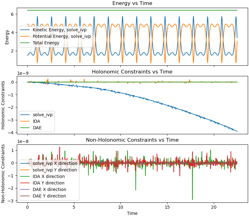
Energy vs Time, Holonomic Constraints vs Time, Non-Holonomic Constraints vs Time

deviation of the total energy from being constant is 7.641e-07 % of max total energy, using solve_ivp
deviation of the total energy from being constant is 5.252e-05 % of max total energy, using IDA
deviation of the total energy from being constant is 6.974e-05 % of max total energy, using DAE


max error in hol. constraint with solve_ivp is 3.909e-09
max error in hol. constraint with IDA is       2.756e-10
max error in hol. constraint with solve_dae is 2.601e-11


max error in non-hol. constraint with solve_ivp is 4.611e-09
max error in non-hol. constraint with IDA is       2.922e-08
max error in non-hol. constraint with solve_dae is 9.157e-10

Animation¶

The animation only runs for the first third of the simulation time, to save space.

fps = 10

# Interpolation of the solution
duration = int(schritte / 3)
tf = resultat1.t[duration-1]
t_arr = np.asarray(resultat1.t[:duration])
y_arr = np.asarray(resultat1.y[:, :duration])

state_sol = interp1d(
    t_arr,
    y_arr,
    kind="cubic",
    axis=1
)

# CP coordinates
CP_vec = CP.pos_from(O)

coordinates = [
    CP_vec.dot(N.x),
    CP_vec.dot(N.y),
    CP_vec.dot(N.z)
]

coords_lam = sm.lambdify(
    qL + pL,
    coordinates,
    cse=True
)

# Plot limits
max_x = np.max(y_arr[3, :]) + r1
max_y = np.max(y_arr[4, :]) + r1
min_x = np.min(y_arr[3, :]) - r1
min_y = np.min(y_arr[4, :]) - r1

max_z = 2 * r1
min_z = -2 * r1

# Disc in x/z plane.
N1 = 80
theta = np.linspace(0, 2*np.pi, N1)

local_disc = np.vstack([
    np.zeros_like(theta),
    r1 * np.cos(theta),
    r1 * np.sin(theta)
])

# Dot on the disc to show rotation.
local_dot = np.array([
    0.0,
    r1,
    0.0
])

# Center of the disc.


def center(t):
    s = np.asarray(state_sol(t)).reshape(-1)
    return np.array([
        s[3],
        s[4],
        s[5]
    ], dtype=float)


# Rotation matrices.
def Rx(a):
    return np.array([
        [1, 0, 0],
        [0, np.cos(a), -np.sin(a)],
        [0, np.sin(a),  np.cos(a)]
    ])


def Ry(a):
    return np.array([
        [np.cos(a), 0, np.sin(a)],
        [0, 1, 0],
        [-np.sin(a), 0, np.cos(a)]
    ])


def Rz(a):
    return np.array([
        [np.cos(a), -np.sin(a), 0],
        [np.sin(a),  np.cos(a), 0],
        [0,          0,         1]
    ])


# Animation frames.
frames = np.arange(t0, tf, 1/fps)

# Precalculate CP trajectory.
traj_full = np.array([
    np.asarray(
        coords_lam(*np.asarray(state_sol(tt)).reshape(-1), *pL_vals),
        dtype=float
    ).reshape(-1)
    for tt in frames
])


# Figure.
fig = plt.figure(figsize=(8, 8), constrained_layout=True)
ax = fig.add_subplot(111, projection="3d")

ax.set_xlim(min_x, max_x)
ax.set_ylim(min_y, max_y)
ax.set_zlim(min_z, max_z)

ax.set_xlabel("X", fontsize=15)
ax.set_ylabel("Y", fontsize=15)
ax.set_zlabel("Z")

# Ground plane.
xx, yy = np.meshgrid(
    np.linspace(min_x, max_x, 2),
    np.linspace(min_y, max_y, 2)
)

zz = np.zeros_like(xx)

ax.plot_surface(
    xx, yy, zz,
    alpha=0.2
)


# Artists
disc, = ax.plot([], [], [], lw=2)
dot, = ax.plot([], [], [], "o", markersize=6)
axle, = ax.plot([], [], [], lw=3)
point, = ax.plot([], [], [], "o", markersize=6)
CP_loc, = ax.plot([], [], [], "o", markersize=6, color='black')

trajectory, = ax.plot(
    [], [], [],
    "--",
    alpha=0.5
)

# Update function


def update(t):

    # Get state as a simple 1D numpy array
    s = np.asarray(state_sol(t)).reshape(-1)

    # Title.
    msg = (
        f"Running time: {float(t):.2f} \n"
        f"The black dot indicates the contact point, \n the green dot only "
        f"shows the rotation of the disc. The red axle just to help \n"
        f"visualize the orientation of the disc. \n"
        "The dotted line shows the trajectory of the contact point"
    )
    ax.set_title(msg, fontsize=12)

    # Center.
    c = np.array(
        [s[3], s[4], s[5]],
        dtype=float
    )

    # Orientation
    qx = float(s[0])
    qy = float(s[1])
    qz = float(s[2])

    R = Rz(qz) @ Ry(qy) @ Rx(qx)

    # Disc
    disc_world = R @ local_disc
    disc_world = disc_world + c[:, None]

    disc.set_data(
        disc_world[0, :],
        disc_world[1, :]
    )

    disc.set_3d_properties(
        disc_world[2, :]
    )

    # Dot
    dot_world = R @ local_dot
    dot_world = dot_world + c

    dot.set_data(
        [dot_world[0]],
        [dot_world[1]]
    )

    dot.set_3d_properties(
        [dot_world[2]]
    )

    # Axle.
    axle_length = r1 * 1.25

    p1 = c - 0.5 * axle_length * R[:, 0]
    p2 = c + 0.5 * axle_length * R[:, 0]

    axle.set_data(
        [p1[0], p2[0]],
        [p1[1], p2[1]]
    )

    axle.set_3d_properties(
        [p1[2], p2[2]]
    )

    # Center
    point.set_data(
        [c[0]],
        [c[1]]
    )

    point.set_3d_properties(
        [c[2]]
    )

    # CP trajectory
    mask = frames <= t

    trajectory.set_data(
        traj_full[mask, 0],
        traj_full[mask, 1]
    )

    trajectory.set_3d_properties(
        traj_full[mask, 2]
    )

    # Current CP position
    coord = np.asarray(
        coords_lam(*s, *pL_vals),
        dtype=float
    ).reshape(-1)

    CP_loc.set_data(
        [coord[0]],
        [coord[1]]
    )

    CP_loc.set_3d_properties(
        [coord[2]]
    )

    return disc, dot, axle, point, trajectory, CP_loc


# Create animation
animation = FuncAnimation(
    fig,
    update,
    frames=frames,
    interval=1000/fps,
    blit=False
)

plt.show()

Total running time of the script: (0 minutes 33.269 seconds)

Gallery generated by Sphinx-Gallery

Glocker and Leine Problem¶

Objective¶

Description¶

Notes¶

Kane’s Equations of Motion.¶

Prepare for solve_dae and for IDA¶

Animation¶

Peter's Mechanics Examples

Navigation

Related Topics