Ellipses Posa 2013

Description

An ellipse which can rotate around its mass center fixed in space is at rest initially. A two-finger design should push the resting ellipse to amimize its final angular speed. The finger part touching this ellipse is also an ellipse. The impact is modeled as a linear spring, the direction normal to the tangent at the contact point. There is no friction.

Notes

• The idea was taken from Posa et.al., A direct Method for Trajectory Optimization of Rigid Bodies Through Contact, 2013.

• The problem turned out to be quite difficult to optimize, despite the simple equations of motion. For many initial conditions, I did not manage to get opty to converge.

• Presumably, the problem is the function giving the distance between the two ellipses. Being nonlinear, it has several ‘solutions’ of which of course only one is correct. It may also not converge at all for some initial guesses.

• Whether gravity is present or not makes no difference.

States

• \(q_1, q_2, q_3\) are the angles of the rod and the two ellipses.

• \(u_1, u_2, u_3\) are the angular velocities of the rod and the two ellipses.

Parameters

• \(l_1\) is the length of the rod.

• \(a_2, b_2\) are the half axes of the first ellipse, the one pushing the second one.

• \(a_3, b_3\) are the half axes of the second ellipse, the one at rest initially

• \(x_3, y_3\) are the coordinates of the center of the second ellipse.

• \(m_1, m_2, m_3\) are the masses of the rod and the two ellipses.

import sympy as sm
import sympy.physics.mechanics as me
import numpy as np
import matplotlib.pyplot as plt
import math
from opty import Problem
from opty.utils import MathJaxRepr
from scipy.optimize import root
from scipy.integrate import solve_ivp
from scipy.interpolate import interp1d
from matplotlib.patches import Ellipse
from matplotlib.animation import FuncAnimation

Set Up the Geometry

N, A1, A2, A3 = sm.symbols('N A1 A2 A3', cls=me.ReferenceFrame)
O, Dmc1, Dmc2, Dmc3 = sm.symbols('O Dmc1 Dmc2 Dmc3', cls=me.Point)
t = me.dynamicsymbols._t
O.set_vel(N, 0)

P0, P1, P2 = sm.symbols('P0 P1 P2', cls=me.Point)
q1, q2, q3 = sm.symbols('q1 q2 q3', cls=me.dynamicsymbols)
u1, u2, u3 = sm.symbols('u1 u2 u3', cls=me.dynamicsymbols)

l1, a2, b2, a3, b3 = sm.symbols('l1, a2 b2 a3 b3')
x3, y3 = sm.symbols('x3 y3')

A1.orient_axis(N, q1, N.z)
A1.set_ang_vel(N, u1 * N.z)
A2.orient_axis(N, q2, N.z)
A3.orient_axis(N, q3, N.z)
A2.set_ang_vel(N, u2 * N.z)
A3.set_ang_vel(N, u3 * N.z)

P0.set_pos(O, 0)
Dmc1.set_pos(P0, -l1/2 * A1.y)
Dmc1.v2pt_theory(P0, N, A1)
P1.set_pos(Dmc1, -l1/2 * A1.y)
P1.v2pt_theory(Dmc1, N, A1)
Dmc2.set_pos(P1, -b2 * A2.y)
Dmc2.v2pt_theory(P1, N, A2)

Dmc3.set_pos(O, x3*N.x + y3*N.y)
Dmc3.set_vel(N, 0)

Find the points on the ellipses with closest distance. Essentially the idea is that the tangents at the points of closest distance are parallel. The routine calculation was done by AI.

phi = me.dynamicsymbols('phi')

Direction of the tangent on the ellipses at the points of closest distance.

norm_vec = -sm.sin(phi) * N.x + sm.cos(phi) * N.y

Normal to tangent, pointing from ellipse3 to ellipse2.

norm_vec1 = sm.cos(phi) * N.x + sm.sin(phi) * N.y

Formulas for the points on the ellipses with closest distance.

rho1 = sm.sqrt(a2**2 * sm.cos(phi - q2)**2 + b2**2 * sm.sin(phi - q2)**2)
rho2 = sm.sqrt(a3**2 * sm.cos(phi - q3)**2 + b3**2 * sm.sin(phi - q3)**2)
c1_h = (sm.Matrix([a2**2 * sm.cos(phi - q2), b2**2 * sm.sin(phi - q2), 0]) /
        rho1)
c2_h = (sm.Matrix([a3**2 * sm.cos(phi - q3), b3**2 * sm.sin(phi - q3), 0]) /
        rho2)

hilfs1 = A2.dcm(N).T * c1_h
hilfs2 = A3.dcm(N).T * c2_h

hilfs1 = hilfs1[0] * N.x + hilfs1[1] * N.y + hilfs1[2] * N.z
hilfs2 = hilfs2[0] * N.x + hilfs2[1] * N.y + hilfs2[2] * N.z

c1 = Dmc2.pos_from(P0) - hilfs1
c2 = Dmc3.pos_from(P0) + hilfs2

phi_null = norm_vec.dot(c2 - c1)
phi_null = phi_null.trigsimp()

Print the nonlinear equation for phi, the angle of the normal at the contact point.

MathJaxRepr(phi_null)

$$- \frac{\sqrt{2} a_{2}^{2} \sin{\left(2 \left(\phi - q_{2}\right) \right)}}{2 \sqrt{a_{2}^{2} \cos{\left(2 \left(\phi - q_{2}\right) \right)} + a_{2}^{2} - b_{2}^{2} \cos{\left(2 \left(\phi - q_{2}\right) \right)} + b_{2}^{2}}} - \frac{\sqrt{2} a_{3}^{2} \sin{\left(2 \left(\phi - q_{3}\right) \right)}}{2 \sqrt{a_{3}^{2} \cos{\left(2 \left(\phi - q_{3}\right) \right)} + a_{3}^{2} - b_{3}^{2} \cos{\left(2 \left(\phi - q_{3}\right) \right)} + b_{3}^{2}}} + \frac{\sqrt{2} b_{2}^{2} \sin{\left(2 \left(\phi - q_{2}\right) \right)}}{2 \sqrt{a_{2}^{2} \cos{\left(2 \left(\phi - q_{2}\right) \right)} + a_{2}^{2} - b_{2}^{2} \cos{\left(2 \left(\phi - q_{2}\right) \right)} + b_{2}^{2}}} + b_{2} \cos{\left(\phi - q_{2} \right)} + \frac{\sqrt{2} b_{3}^{2} \sin{\left(2 \left(\phi - q_{3}\right) \right)}}{2 \sqrt{a_{3}^{2} \cos{\left(2 \left(\phi - q_{3}\right) \right)} + a_{3}^{2} - b_{3}^{2} \cos{\left(2 \left(\phi - q_{3}\right) \right)} + b_{3}^{2}}} + l_{1} \cos{\left(\phi - q_{1} \right)} - x_{3} \sin{\left(\phi \right)} + y_{3} \cos{\left(\phi \right)}$$

Pick the geometric initial values.

Note: distanz is signed: It is < 0 if the ellipses penetrate.

q11 = np.deg2rad(20.0)
q21 = np.deg2rad(45.0)
q31 = np.deg2rad(0.0)

l11 = 4.0
a21 = 1.0
b21 = 3.0
a31 = 1.0
b31 = 2.0

x31 = 2.52
y31 = -10.0

pL = [q1, q2, q3, l1, a2, b2, a3, b3, x3, y3]
pL_vals = [q11, q21, q31, l11, a21, b21, a31, b31, x31, y31]

phi_null_lam = sm.lambdify([phi] + pL, phi_null, cse=True)
c1_lam = sm.lambdify([phi] + pL, [c1.dot(N.x), c1.dot(N.y)], cse=True)
c2_lam = sm.lambdify([phi] + pL, [c2.dot(N.x), c2.dot(N.y)], cse=True)

distanz = (Dmc2.pos_from(O) - Dmc3.pos_from(O)).dot(norm_vec1) + (-rho1 - rho2)
distanz_lam = sm.lambdify([phi] + pL, distanz, cse=True)
distanz_direct = (c1 - c2).magnitude()
distanz_direct_lam = sm.lambdify([phi] + pL, distanz_direct, cse=True)


def phi_null_func(x0, args):
    return phi_null_lam(x0, *args)

As there are several possible solutions, we need to specify the initial guess carefully.

initial_value = -5.0
res = root(phi_null_func, initial_value, args=(pL_vals,))
print(res.message)
phi1 = math.fmod(res.x[0], 2.0 * np.pi)
phi1

The solution converged.

-5.375874348448542

\(c_1, c_2\) are definded without reference to the respective ellipses. They are vectors.

\(c_{1e}, c_{2e}\) are points definded w.r.t. the ellipses to be same points in space.

c1e, c1eh = me.Point('c1e'), me.Point('c1eh')
c2e, c2eh = me.Point('c2e'), me.Point('c2eh')

vector_Dmc3 = c2 - Dmc3.pos_from(P0)
c2e.set_pos(Dmc3, vector_Dmc3)
c2eh.set_pos(c2e, norm_vec1)

vector_Dmc2 = c1 - Dmc2.pos_from(P0)
c1e.set_pos(Dmc2, vector_Dmc2)
c1eh.set_pos(c1e, norm_vec1)

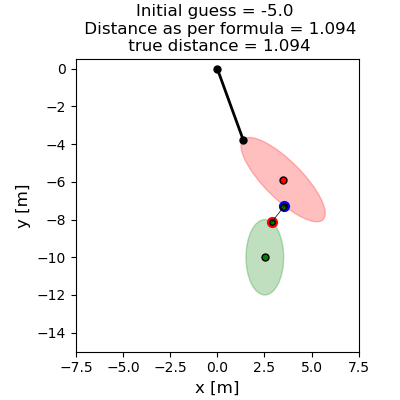
Visualize initial condition. Ensure the formulae give results as expected.

def plot_initial_config(ax, initial_value, phi1, c1e, c2e, c2eh):

    coords = Dmc1.pos_from(P0).to_matrix(N)
    for point in (Dmc2, Dmc3, P1, c1e, c2e, c2eh):
        coords = coords.row_join(point.pos_from(P0).to_matrix(N))

    coords_lam = sm.lambdify([phi] + pL, coords, cse=True)
    coords_vals = coords_lam(phi1, *pL_vals)

    c1_vals = c1_lam(phi1, *pL_vals)
    c2_vals = c2_lam(phi1, *pL_vals)

    ellipse2 = Ellipse(
        (coords_vals[0, 1], coords_vals[1, 1]),  # center
        width=2*a21,        # full width = 2a
        height=2*b21,       # full height = 2b
        angle=np.rad2deg(q21),          # rotation in degrees
        facecolor='red',
        edgecolor='red',
        alpha=0.25,
    )

    ellipse3 = Ellipse(
        (coords_vals[0, 2], coords_vals[1, 2]),  # center
        width=2*a31,        # full width = 2a
        height=2*b31,       # full height = 2b
        angle=np.rad2deg(q31),          # rotation in degrees
        facecolor='green',
        edgecolor='green',
        alpha=0.25,
    )

    ax.add_patch(ellipse2)
    ax.add_patch(ellipse3)

    ax.plot([0.0, coords_vals[0, 3]], [0.0, coords_vals[1, 3]], color='black',
            linestyle='-', lw=2.0)
    ax.plot([c1_vals[0], c2_vals[0]], [c1_vals[1], c2_vals[1]], color='black',
            linestyle='-', lw=0.5)
    ax.scatter(c1_vals[0], c1_vals[1], color='blue', s=50)
    ax.scatter(c2_vals[0], c2_vals[1], color='red', s=50)
    ax.scatter(0.0, 0.0, color='black', s=25)
    ax.scatter(coords_vals[0, 3], coords_vals[1, 3], color='black', s=25)
    ax.scatter(coords_vals[0, 1], coords_vals[1, 1], color='red', s=25,
               edgecolor='black')
    ax.scatter(coords_vals[0, 2], coords_vals[1, 2], color='green', s=25,
               edgecolor='black')
    ax.scatter(coords_vals[0, 4], coords_vals[1, 4], color='red', s=15,
               edgecolor='black')
    ax.scatter(coords_vals[0, 5], coords_vals[1, 5], color='green', s=15,
               edgecolor='black')
    ax.scatter(coords_vals[0, 6], coords_vals[1, 6], color='green', s=15,
               edgecolor='black')

    ax.set_aspect('equal')
    ax.set_xlim(-7.5, 7.5)
    ax.set_ylim(-15, 0.5)
    ax.set_xlabel('x [m]', fontsize=12)
    ax.set_ylabel('y [m]', fontsize=12)
    ax.set_title(f"Initial guess = {initial_value} \n "
                 f"Distance as per formula = {distanz_lam(phi1, *pL_vals):.3f}"
                 "\n "
                 f"true distance = {distanz_direct_lam(phi1, *pL_vals):.3f}",
                 fontsize=12)


fig, ax = plt.subplots(figsize=(4, 4), layout='constrained')
plot_initial_config(ax, initial_value, phi1, c1e, c2e, c2eh)

Show the effect of different initial guesses on the location of the contact points and their distance. True distance is the geometric distance between the points \(c_1, c_2\)

fig, axen = plt.subplots(1, 3, figsize=(12, 4), layout='constrained')

for axis, initial_value in enumerate([-5.0, 5.0, -15.0]):
    res = root(phi_null_func, initial_value, args=(pL_vals,))
    print(f"with initial value {initial_value}: {res.message}")
    phi1_h = math.fmod(res.x[0], 2.0 * np.pi)

    c1e_h, c1eh_h = me.Point('c1e_h'), me.Point('c1eh_h')
    c2e_h, c2eh_h = me.Point('c2e_h'), me.Point('c2eh_h')

    vector_Dmc3 = c2 - Dmc3.pos_from(P0)
    c2e_h.set_pos(Dmc3, vector_Dmc3)
    c2eh_h.set_pos(c2e_h, norm_vec1)

    vector_Dmc2 = c1 - Dmc2.pos_from(P0)
    c1e_h.set_pos(Dmc2, vector_Dmc2)
    c1eh_h.set_pos(c1e_h, norm_vec1)
    plot_initial_config(axen[axis], initial_value, phi1_h, c1e_h, c2e_h,
                        c2eh_h)

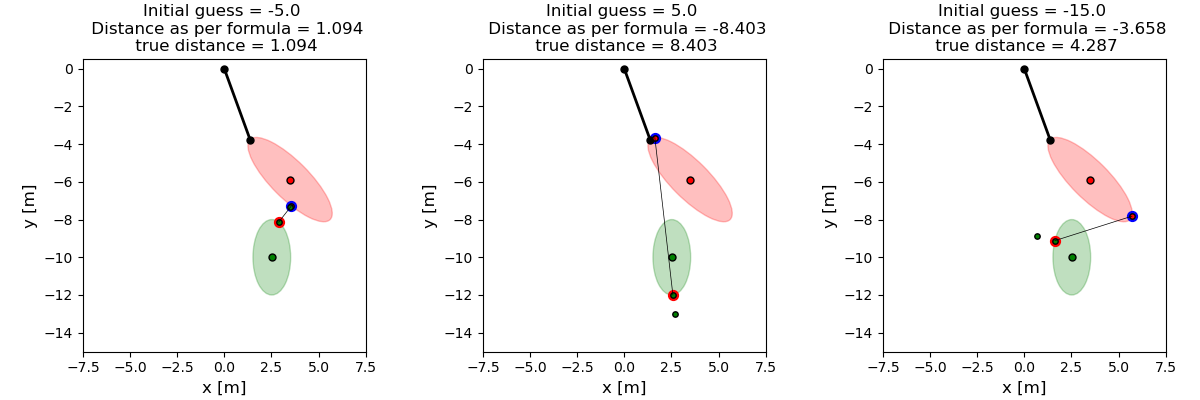
with initial value -5.0: The solution converged.
with initial value 5.0: The solution converged.
with initial value -15.0: The iteration is not making good progress, as measured by the
 improvement from the last ten iterations.

Set up Kane’s Equations

Control torques.

T1, T2 = me.dynamicsymbols('T1 T2')

Function have the contact forces act only when the ellipses penetrate.

def smooth_step(xx, aa, steep=50):
    """returns 1 for xx << aa, 0 for xx >> aa."""
    return 0.5 * (1 - sm.tanh(steep * (xx - aa)))

Finish up Kane’s equations.

m1, m2, m3, g, k_spring = sm.symbols('m1 m2 m3 g k_spring')

iZZ1 = 1/12 * m1 * l1**2  # inertia of the rod about its center
iZZ2 = 1/4 * m2 * (a2**2 + b2**2)  # inertia of the ellipse about its center
iZZ3 = 1/4 * m3 * (a3**2 + b3**2)  # inertia of the ellipse about its center

inert1 = me.inertia(A1, 0, 0, iZZ1)
inert2 = me.inertia(A2, 0, 0, iZZ2)
inert3 = me.inertia(A3, 0, 0, iZZ3)

rod1 = me.RigidBody('rod1', Dmc1, A1, m1, (inert1, Dmc1))
elli2 = me.RigidBody('elli2', Dmc2, A2, m2, (inert2, Dmc2))
elli3 = me.RigidBody('elli3', Dmc3, A3, m3, (inert3, Dmc3))
bodies = [rod1, elli2, elli3]

FL1 = [(Dmc1, -m1 * g * N.y), (Dmc2, -m2 * g * N.y), (Dmc3, -m3 * g * N.y)]
TL1 = [(A1, T1*N.z), (A2, T2*N.z)]
FL_impact = [(c1e, -k_spring * distanz * smooth_step(distanz, 0.0) *
              norm_vec1),
             (c2e, k_spring * distanz * smooth_step(distanz, 0.0) *
              norm_vec1)]
forces = FL1 + TL1 + FL_impact

kd = sm.Matrix([q1.diff(t) - u1, q2.diff(t) - u2, q3.diff(t) - u3])

q_ind = [q1, q2, q3]
u_ind = [u1, u2, u3]

kane = me.KanesMethod(N, q_ind, u_ind, kd_eqs=kd)
fr, frstar = kane.kanes_equations(bodies, forces)

eom = kd.col_join(fr + frstar)

the solution of phi_null = 0 gives phi.

eom = eom.col_join(sm.Matrix([phi_null]))

Prevent too much penetration. Without some restriction I did not get it to converge.

eom = eom.col_join(sm.Matrix([distanz]))

Print some information about the equations of motion for opty.

print(f"eom contain {sm.count_ops(eom)} operations")
print(f"eom contain {len(eom)} equations")
print('eom dynamic symbols:', me.find_dynamicsymbols(eom))
print('eom free symbols:', eom.free_symbols, '\n')

eom contain 2472 operations
eom contain 8 equations
eom dynamic symbols: {phi(t), Derivative(u3(t), t), u3(t), u1(t), Derivative(q2(t), t), T2(t), Derivative(q1(t), t), T1(t), Derivative(u1(t), t), q2(t), Derivative(q3(t), t), q1(t), q3(t), u2(t), Derivative(u2(t), t)}
eom free symbols: {y3, t, g, m1, m3, x3, b2, k_spring, a2, b3, a3, m2, l1}

Adopt for numerical integration:

• remove \(T_1, T_2\).

• form \(f_r, f_r^{\star}\) again, with the reduced force list.

• create mass matrix and forcing vector.

forces = FL1 + FL_impact
fr1, frstar1 = kane.kanes_equations(bodies, forces)
MM = kane.mass_matrix_full
force = kane.forcing_full

Print some information about the equations of motion for the numerical integration.

print(f"force contains {sm.count_ops(force)} operations")
print(f"force contain {len(force)} equations")
print('force dynamic symbols:', me.find_dynamicsymbols(force))
print('force free symbols:', force.free_symbols, '\n')

print(f"MM contains {sm.count_ops(MM)} operations")
print(f"MM contain {len(MM)} equations")
print('MM dynamic symbols:', me.find_dynamicsymbols(MM))
print('MM free symbols:', MM.free_symbols)

force contains 2167 operations
force contain 6 equations
force dynamic symbols: {phi(t), u1(t), u3(t), q3(t), q1(t), u2(t), q2(t)}
force free symbols: {y3, t, g, m1, x3, b2, k_spring, a2, b3, a3, m2, l1}

MM contains 47 operations
MM contain 36 equations
MM dynamic symbols: {q2(t), q1(t)}
MM free symbols: {b2, a2, t, b3, a3, m1, m2, l1, m3}

Compilation

qL = q_ind + u_ind
pL = [phi, l1, a2, b2, a3, b3, x3, y3, m1, m2, m3, g, k_spring]

MM_lam = sm.lambdify(qL + pL, MM, cse=True)
force_lam = sm.lambdify(qL + pL, force, cse=True)

Numerical Integration.

Done to ensure the equations of motion match mechanical intuition.

m11 = l11
m21 = np.pi * a21 * b21
m31 = np.pi * a31 * b31
g1 = 9.81

u11 = 0.0
u21 = 0.0
u31 = 4.0
k_spring1 = 6000.0

t0, tf = 0.0, 3.0

punkte = 50
schritte = int(tf * punkte)
times = np.linspace(t0, tf, schritte)

pL_vals = [phi1, l11, a21, b21, a31, b31, x31, y31,
           m11, m21, m31, g1, k_spring1]
y0 = np.array([q11, q21, q31, u11, u21, u31])

# pL = [q1, q2, q3, l1, a2, b2, a3, b3, x3, y3]

phi_list = []
t_list = []
zaehler = 0


def gradient(t, y, args):
    global zaehler

    x0 = args[0]
    args1 = list(y[0: 3]) + list(args[1: 8])
    res = root(phi_null_func, x0, args1)
    if not res.success:
        zaehler += 1
    args[0] = res.x[0]
    phi_list.append(res.x[0])
    t_list.append(t)

    sol = np.linalg.solve(MM_lam(*y, *args), force_lam(*y, *args))
    return np.array(sol).squeeze()


t_span = (0., tf)
resultat1 = solve_ivp(gradient, t_span, y0, t_eval=times, args=(pL_vals,),
                      method='Radau',
                      atol=1.e-6,
                      rtol=1.e-6,
                      )

resultat = resultat1.y.T
print(resultat.shape)
print(resultat1.message, resultat1.t[-1])

print('resultat shape', resultat.shape, '\n')

print("To numerically integrate an intervall of {} sec, the routine cycled {} "
      "times".format(tf, resultat1.nfev))

print(f"Number of times root solver failed: {zaehler}")

(150, 6)
The solver successfully reached the end of the integration interval. 3.0
resultat shape (150, 6)

To numerically integrate an intervall of 3.0 sec, the routine cycled 1656 times
Number of times root solver failed: 0

Find the index in t_list closest to resultat1.t. This is needed to select the phi values in phi_list closest to the ones used in resultat.

def nearest_indices(A, B):
    A = np.asarray(A)
    B = np.asarray(B)

    # Find insertion positions
    idx = np.searchsorted(A, B)

    # Clip to valid range
    idx = np.clip(idx, 1, len(A)-1)

    # Compare neighbors
    left = A[idx - 1]
    right = A[idx]

    # Choose closer one
    idx -= (B - left) <= (right - B)

    return idx


idx_values = nearest_indices(t_list, resultat1.t)

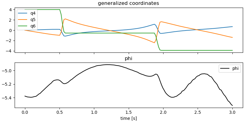
Plot some results.

phi_np = np.array([phi_list[i] for i in idx_values])

fig, ax = plt.subplots(2, 1, figsize=(8, 4), sharex=True, layout='constrained')
for i in range(3, 6):
    ax[0].plot(resultat1.t, resultat[:, i], label=f'q{i+1}')
ax[0].set_title('generalized coordinates')

ax[1].plot(resultat1.t, phi_np, label='phi', color='black')
ax[1].set_title('phi')
ax[0].legend()
ax[1].legend()
_ = ax[1].set_xlabel('time [s]')

Animation

def animateur(resultat, phi_np, t0, tf, schritte):
    """
    returns the animation.
    resultat in the shape time steps x 6 (q1, q2, q3, u1, u2, u3)
    phi_np in the shape time steps (phi)
    """

    fps = 20

    t_arr = np.linspace(t0, tf, schritte)
    state_sol = interp1d(t_arr, resultat, kind='cubic', axis=0)
    input_sol = interp1d(t_arr, phi_np, kind='cubic', axis=0)

    coords = Dmc1.pos_from(P0).to_matrix(N)
    for point in (Dmc2, Dmc3, P1, c1e, c2e):
        coords = coords.row_join(point.pos_from(P0).to_matrix(N))

    pL = [l1, a2, b2, a3, b3, x3, y3]
    pL_vals = [l11, a21, b21, a31, b31, x31, y31]
    qL = [q1, q2, q3, phi]
    coords_lam = sm.lambdify(qL + pL, coords, cse=True)
    coords_vals = coords_lam(*resultat[0, 0: 3], phi_np[0], *pL_vals)

    coords = Dmc1.pos_from(P0).to_matrix(N)
    for point in (Dmc2, Dmc3, P1, c1e, c2e, c2eh):
        coords = coords.row_join(point.pos_from(P0).to_matrix(N))

    coords_lam = sm.lambdify(qL + pL, coords, cse=True)
    coords_vals = coords_lam(*resultat[0, 0: 3], phi_np[0], *pL_vals)

    fig, ax = plt.subplots(figsize=(8, 8))

    ellipse2 = Ellipse(
        (coords_vals[0, 1], coords_vals[1, 1]),          # center
        width=2*a21,        # full width = 2a
        height=2*b21,       # full height = 2b
        angle=np.rad2deg(resultat[0, 1]),          # rotation in degrees
        facecolor='red',
        edgecolor='red',
        alpha=0.25,
    )

    ellipse3 = Ellipse(
        (coords_vals[0, 2], coords_vals[1, 2]),          # center
        width=2*a31,        # full width = 2a
        height=2*b31,       # full height = 2b
        angle=np.rad2deg(resultat[0, 2]),          # rotation in degrees
        facecolor='blue',
        edgecolor='blue',
        alpha=0.25,
    )

    # point of attachment
    ax.scatter(0.0, 0.0, color='black', s=25)
    # end of rod
    line2 = ax.scatter(coords_vals[0, 3], coords_vals[1, 3], color='black',
                       s=25)
    # centers of ellipses
    line3 = ax.scatter(coords_vals[0, 1], coords_vals[1, 1], color='red', s=25,
                       edgecolor='black')
    line4 = ax.scatter(coords_vals[0, 2], coords_vals[1, 2], color='green',
                       s=25, edgecolor='black')
    # contact points
    line5 = ax.scatter(coords_vals[0, 4], coords_vals[1, 4], color='red', s=15,
                       edgecolor='black')
    line6 = ax.scatter(coords_vals[0, 5], coords_vals[1, 5], color='green',
                       s=15, edgecolor='black')

    # the rod
    line7, = ax.plot([0.0, coords_vals[0, 3]], [0.0, coords_vals[1, 3]],
                     color='black',  linestyle='-', lw=2.0)

    # the line between contact points
    line8, = ax.plot([coords_vals[0, 4], coords_vals[0, 5]],
                     [coords_vals[1, 4], coords_vals[1, 5]], color='black',
                     linestyle='-', lw=0.5)

    ax.add_patch(ellipse2)
    ax.add_patch(ellipse3)

    # Set limits
    ax.set_xlim(-7.5, 7.5)
    ax.set_ylim(-15, 0.5)
    ax.set_aspect('equal')
    ax.set_xlabel('x [m]', fontsize=15)
    ax.set_ylabel('y [m]', fontsize=15)

    # Animation update function

    def update(frame):
        t = frame

        ax.set_title(f"Running time: {t:.2f} s")
        coords_vals = coords_lam(*state_sol(t)[0: 3], input_sol(t), *pL_vals)
        # Update ellipse position
        ellipse2.center = (coords_vals[0, 1], coords_vals[1, 1])
        ellipse3.center = (coords_vals[0, 2], coords_vals[1, 2])
        # Rotate ellipse
        ellipse2.angle = np.rad2deg(state_sol(t)[1])
        ellipse3.angle = np.rad2deg(state_sol(t)[2])

        line2.set_offsets((coords_vals[0, 3], coords_vals[1, 3]))
        line3.set_offsets((coords_vals[0, 1], coords_vals[1, 1]))
        line4.set_offsets((coords_vals[0, 2], coords_vals[1, 2]))
        line5.set_offsets((coords_vals[0, 4], coords_vals[1, 4]))
        line6.set_offsets((coords_vals[0, 5], coords_vals[1, 5]))
        line7.set_data([0.0, coords_vals[0, 3]], [0.0, coords_vals[1, 3]])
        line8.set_data([coords_vals[0, 4], coords_vals[0, 5]],
                       [coords_vals[1, 4], coords_vals[1, 5]])

        return (ellipse2, ellipse3, line2, line3, line4, line5, line6,
                line7, line8)

    # Create animation

    ani = FuncAnimation(fig, update, frames=np.arange(0, tf, 1.0/fps),
                        interval=1500/fps, blit=False)
    return ani


anim = animateur(resultat, phi_np, t0=0.0, tf=tf, schritte=schritte)
plt.show()

Once Loop Reflect

Set Up the Optimization

state_symbols = [q1, q2, q3, u1, u2, u3]
num_nodes = schritte
t0 = 0.0
tf = tf
interval_value = (tf - t0) / (num_nodes - 1)

par_map = {}
par_map[m1] = m11
par_map[m2] = m21
par_map[m3] = m31
par_map[g] = g1
par_map[k_spring] = k_spring1
par_map[l1] = l11
par_map[a2] = a21
par_map[b2] = b21
par_map[a3] = a31
par_map[b3] = b31
par_map[x3] = x31
par_map[y3] = y31


def obj(free):
    """maximize the final rotational speed of the ellipse, u3"""
    return -free[6*num_nodes-1]**2


def obj_grad(free):
    """gradient of the objective function"""
    grad = np.zeros_like(free)
    grad[6*num_nodes-1] = -2 * free[6*num_nodes-1]
    return grad


instance_constraints = (
    q1.func(t0) - q11,
    q2.func(t0) - q21,
    q3.func(t0) - q31,
    phi.func(t0) - phi1,
    u1.func(t0) - u11,
    u2.func(t0) - u21,
    u3.func(t0) - 0.0,
)

limit = 100.0
bounds = {
    T1: (-limit, limit),
    T2: (-limit, limit),
    q1: (-np.pi/4, np.pi/4),
    q2: (-np.pi/4, np.pi/4),
}

Prevent too much penetration.

eom_bounds = {
    7: (-0.1, 10),
}

Set up the Problem.

prob = Problem(
    obj,
    obj_grad,
    eom,
    state_symbols,
    num_nodes,
    interval_value,
    known_parameter_map=par_map,
    instance_constraints=instance_constraints,
    bounds=bounds,
    eom_bounds=eom_bounds,
    time_symbol=t,
)

print('sequence of inputs', prob.collocator.current_discrete_specified_symbols)

sequence of inputs (T1i, T2i, phii)

Solve the optimization

initial_guess = np.ones(prob.num_free)
prob.add_option('max_iter', 60000)

solution, info = prob.solve(initial_guess)
print(info['status_msg'])
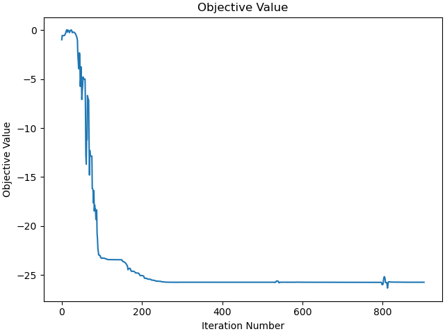
print(f"objective value: {info['obj_val']}")

b'Algorithm terminated successfully at a locally optimal point, satisfying the convergence tolerances (can be specified by options).'
objective value: -25.719716482250096

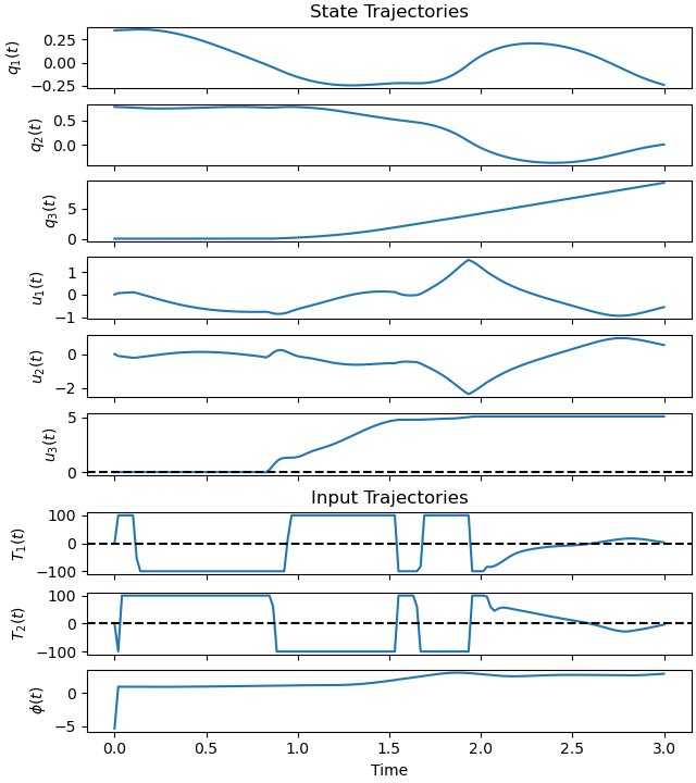
Plot the trajectories.

ax = prob.plot_trajectories(solution)
ax[-2].axhline(0.0, color='black', linestyle='--')
ax[-3].axhline(0.0, color='black', linestyle='--')
_ = ax[5].axhline(0.0, color='black', linestyle='--')

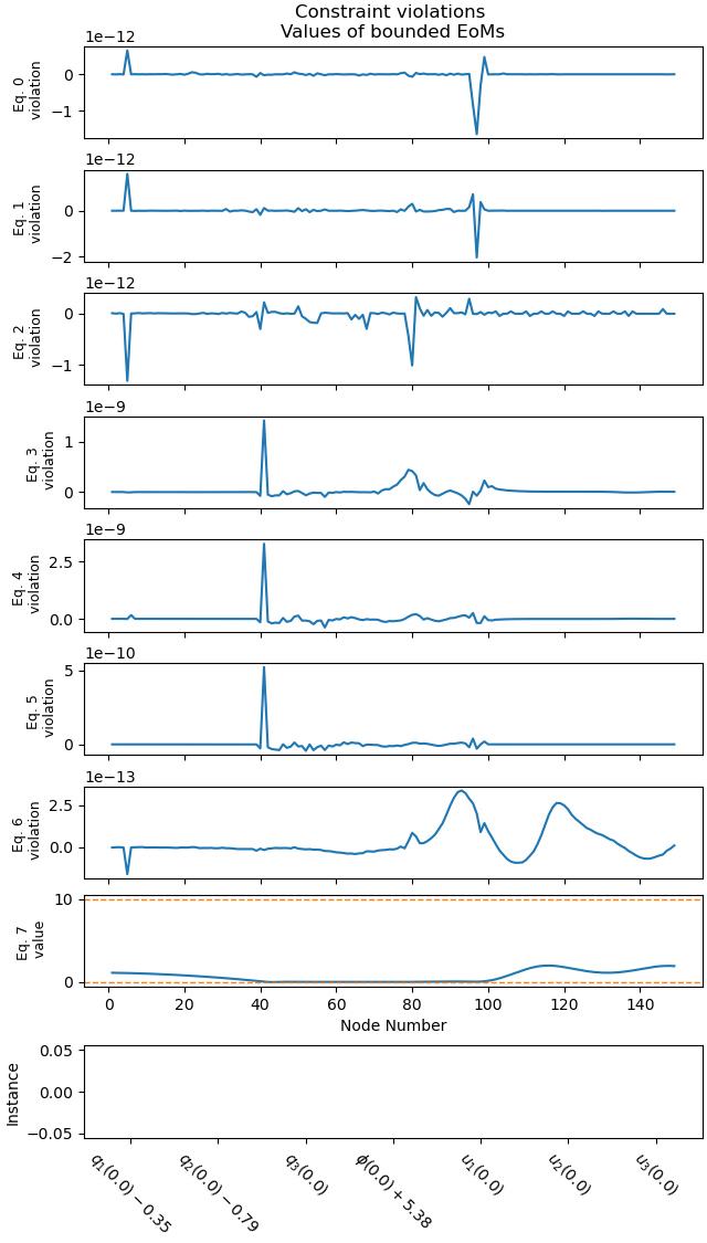
Plot the errors.

_ = prob.plot_constraint_violations(solution, subplots=True, show_bounds=True)

Plot the objective value.

_ = prob.plot_objective_value()

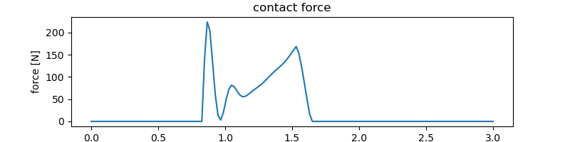
Force between ellipses.

res, inp, *_ = prob.parse_free(solution)
res = res.T
inp = inp.T

distance_values = distanz_lam(inp[:, 2], res[:, 0], res[:, 1],  res[:, 2],
                              l11, a21, b21, a31, b31, x31, y31)
distance_np = -(k_spring1 * distance_values *
                (1.0 - np.heaviside(distance_values, 0.0)))

fig, ax = plt.subplots(figsize=(8, 2))
zeit = np.linspace(t0, tf, schritte)
ax.plot(zeit, distance_np)
ax.set_title('contact force')
ax.set_xlabel('time [s]')
_ = ax.set_ylabel('force [N]')

Animation

resultat, inputs, *_ = prob.parse_free(solution)
resultat = resultat.T
phi_np = inputs[2, :]

ani = animateur(resultat, phi_np, t0=0.0, tf=tf, schritte=schritte)
plt.show()

Once Loop Reflect