Van der Pol Oscillator (Betts 10.144 / 145)

https://en.wikipedia.org/wiki/Van_der_Pol_oscillator

These are examples 10.144 / 145 from John T. Betts, Practical Methods for Optimal Control Using NonlinearProgramming, 3rd edition, Chapter 10: Test Problems. It is described in more detail in section 4.14. example 4.11 of the book.

Note

• A rather high number of nodes is required to get a good solution. Maybe an indication that the problem is stiff.

• Both formulations give very similar results.

import numpy as np
import sympy as sm
import sympy.physics.mechanics as me
import time
from opty.direct_collocation import Problem
from opty.utils import create_objective_function, MathJaxRepr
import matplotlib.pyplot as plt

First version of the problem (10.144)

States

\(y_1, y_2\) : state variables

Controls

\(u\) : control variables

Equations of Motion.

t = me.dynamicsymbols._t

y1, y2 = me.dynamicsymbols('y1, y2')
u = me.dynamicsymbols('u')

eom = sm.Matrix([
    -y1.diff() + y2,
    -y2.diff(t) + (1 - y1**2)*y2 - y1 + u,
])

MathJaxRepr(eom)

$$\left[\begin{matrix}y_{2} - \dot{y}_{1}\\\left(1 - y_{1}^{2}\right) y_{2} + u - y_{1} - \dot{y}_{2}\end{matrix}\right]$$

Define and Solve the Optimization Problem.

num_nodes = 20001

t0, tf = 0.0, 5.0
interval_value = (tf - t0) / (num_nodes - 1)

state_symbols = (y1, y2)
unkonwn_input_trajectories = (u, )

objective = sm.integrate(u**2 + y1**2 + y2**2, t)
obj, obj_grad = create_objective_function(
    objective,
    state_symbols,
    unkonwn_input_trajectories,
    tuple(),
    num_nodes,
    interval_value,
    time_symbol=t
)

instance_constraints = (
        y1.func(t0) - 1.0,
        y2.func(t0),
)

bounds = {
        y2: (-0.4, np.inf),
}

prob = Problem(
    obj,
    obj_grad,
    eom,
    state_symbols,
    num_nodes,
    interval_value,
    instance_constraints=instance_constraints,
    bounds=bounds,
    time_symbol=t,
)

Solve the optimization problem. Give some rough estimates for the trajectories.

initial_guess = np.ones(prob.num_free)

Find the optimal solution.

start = time.time()
solution, info = prob.solve(initial_guess)
end = time.time()
print(f"Solving took {end - start:.2f} seconds.")
print(info['status_msg'])
Jstar = 2.95369916
print(f"Objectve is: {info['obj_val']:.8f}, " +
      f"as per the book it is {Jstar}, so the deviation is: "
      f"{(info['obj_val'] - Jstar) / Jstar * 100:.5e} %")

Solving took 4.67 seconds.
b'Algorithm terminated successfully at a locally optimal point, satisfying the convergence tolerances (can be specified by options).'
Objectve is: 2.95319329, as per the book it is 2.95369916, so the deviation is: -1.71266e-02 %

Store the first solution for later comparison.

solution1 = solution

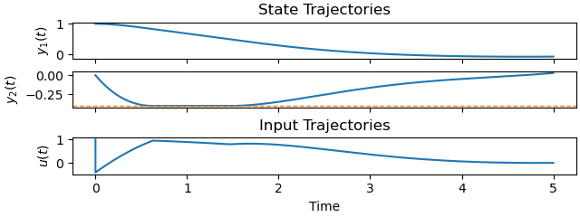
Plot the optimal state and input trajectories.

_ = prob.plot_trajectories(solution, show_bounds=True)

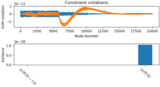
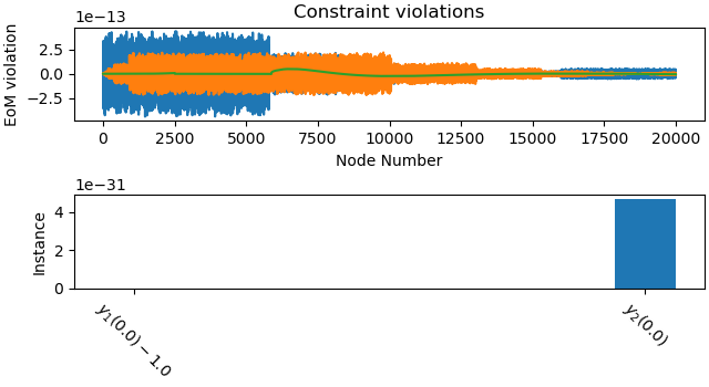
Plot the constraint violations.

_ = prob.plot_constraint_violations(solution)

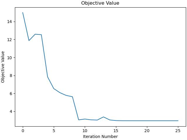
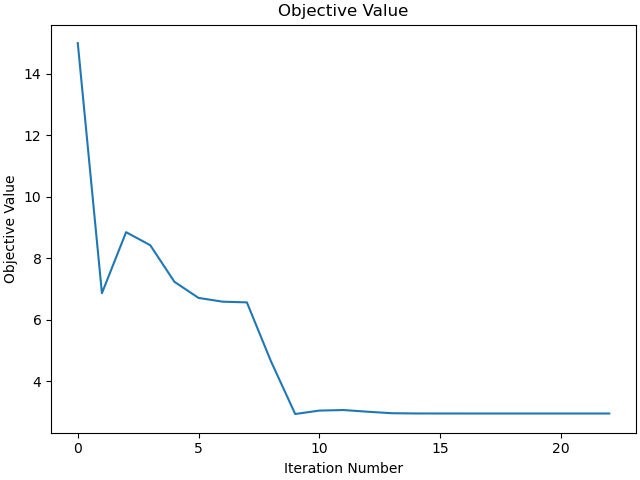
Plot the objective function as a function of optimizer iteration.

_ = prob.plot_objective_value()

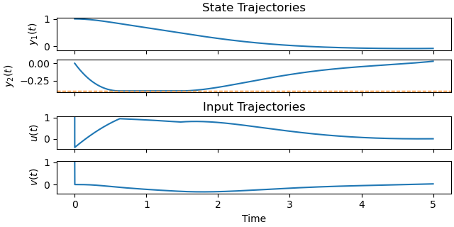
Second version of the problem (10.145)

It is same as problem 10.144 but reformulated. It has two control variables and one additional algebraic equation of motion.

States

\(y_1, y_2\) : state variables

Controls

\(u, v\) : control variables

Equations of Motion.

y1, y2, v = me.dynamicsymbols('y1, y2, v')
u = me.dynamicsymbols('u')

eom = sm.Matrix([
    -y1.diff() + y2,
    -y2.diff(t) + v - y1 + u,
    v - (1-y1**2)*y2,
])
MathJaxRepr(eom)

$$\left[\begin{matrix}y_{2} - \dot{y}_{1}\\u + v - y_{1} - \dot{y}_{2}\\- \left(1 - y_{1}^{2}\right) y_{2} + v\end{matrix}\right]$$

Define and Solve the Optimization Problem

state_symbols = (y1, y2)
unkonwn_input_trajectories = (u, v)

objective = sm.integrate(u**2 + y1**2 + y2**2, t)
obj, obj_grad = create_objective_function(
    objective,
    state_symbols,
    unkonwn_input_trajectories,
    tuple(),
    num_nodes,
    interval_value
)

instance_constraints = (
        y1.func(t0) - 1.0,
        y2.func(t0),
)

bounds = {
        y2: (-0.4, np.inf),
}

prob = Problem(
    obj,
    obj_grad,
    eom,
    state_symbols,
    num_nodes,
    interval_value,
    instance_constraints=instance_constraints,
    bounds=bounds,
    time_symbol=t,
)

Solve the optimization problem. Give some rough estimates for the trajectories.

initial_guess = np.ones(prob.num_free)

Find the optimal solution.

start = time.time()
solution, info = prob.solve(initial_guess)
end = time.time()
print(f"Solving took {end - start:.2f} seconds.")
Jstar = 2.95369916
print(f"Objectve is: {info['obj_val']:.8f}, " +
      f"as per the book it is {Jstar}, so the deviation is: "
      f"{(info['obj_val'] - Jstar) / Jstar * 100:.5e} %")

Solving took 6.36 seconds.
Objectve is: 2.95319329, as per the book it is 2.95369916, so the deviation is: -1.71266e-02 %

Plot the optimal state and input trajectories.

_ = prob.plot_trajectories(solution, show_bounds=True)

Plot the constraint violations.

_ = prob.plot_constraint_violations(solution)

Plot the objective function as a function of optimizer iteration.

_ = prob.plot_objective_value()

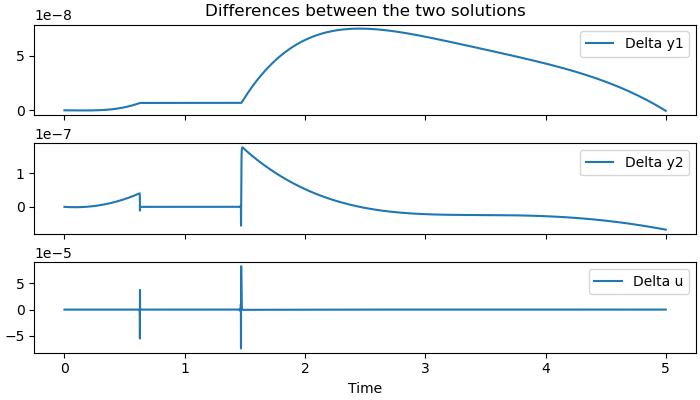
Plot the Difference between the two Solutions.

diffy1 = solution1[: num_nodes] - solution[: num_nodes]
diffy2 = solution1[num_nodes: 2*num_nodes] - solution[num_nodes: 2*num_nodes]
diffu = solution1[2*num_nodes:] - solution[2*num_nodes: 3*num_nodes]
times = np.linspace(t0, tf, num_nodes)

fig, ax = plt.subplots(3, 1, figsize=(7, 4), sharex=True,
                       constrained_layout=True)
ax[0].plot(times, diffy1, label='Delta y1')
ax[0].legend()
ax[1].plot(times, diffy2, label='Delta y2')
ax[1].legend()
ax[2].plot(times, diffu, label='Delta u')
ax[2].legend()
ax[2].set_xlabel('Time')
_ = ax[0].set_title('Differences between the two solutions')