Light Ray in Non-Homogeneous Medium

Description.

A light ray travels from A to B in a non-homogeneous 2D medium. As per Fermat’s principle, the light ray will follow the path that minimizes the travel time.

It is solved in two different ways:

• Variational approach using Euler’s equations, and using solve_bvp for the boundary value problem.

• Let opty find the best way for the light ray. Here numerical trajectories are used to show their use in a simple problem.

Notes

• Currently opty does not allow numerical trajectories to depend on more than one variable, see opty issue #494. So two separate numerical trajectories must be defined. This causes the constraint equation of the eoms to look a bit complicated.

• For some reason, only backend='numpy' works, backend='cython' raises an error, see opty issue #558. As opty converges very fast with this simulation is not a problem.

• Of course, this simulation would have worked without using numerical trajectories, they are used here to demonstrate how to use them.

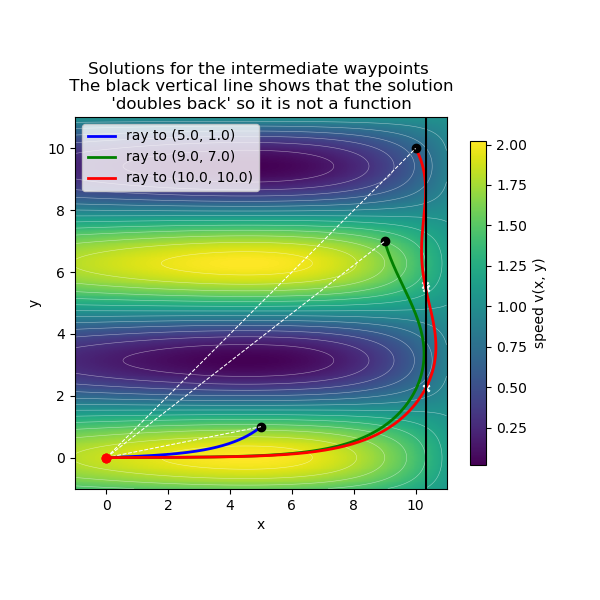
• The optimal trajectory ‘reverses itself’, so it cannot be described as a function y(x), but must be described parametrically as \(x(\tau), y(\tau)\) in the variational formulation. (With opty it is described like this anyway)

• This simple example shows, that both opty and the classical variational approach only find local stationary solutions (variational method) or local minimal solution (opty): changing way_points or initial guesses can lead to very different solutions.

• Increasing fps in the animation will make the motion smoother, but at the expense of increase storage requirements.

import sympy as sm
import sympy.physics.mechanics as me
import numpy as np
import matplotlib.pyplot as plt

from opty import Problem
from scipy.integrate import solve_bvp
from scipy.interpolate import CubicSpline
from matplotlib.animation import FuncAnimation

Define the scalar speed field.

constant = 1.02
ox, oy = sm.symbols('ox oy')


def scalar_x(ox):
    return sm.sin(sm.exp(0.1 * ox))


def scalar_y(oy):
    return sm.cos(oy)


def scalar_speed_field(ox, oy):
    return scalar_x(ox) * scalar_y(oy) + constant


speed_field_lam = sm.lambdify((ox, oy), scalar_speed_field(ox, oy))
scalar_x_lam = sm.lambdify(ox, scalar_x(ox))
scalar_y_lam = sm.lambdify(oy, scalar_y(oy))

speed_field_dx = scalar_x(ox).diff(ox)
speed_field_dy = scalar_y(oy).diff(oy)

speed_field_dx_lam = sm.lambdify((ox), speed_field_dx)
speed_field_dy_lam = sm.lambdify((oy), speed_field_dy)

Variational Problem

A light ray travels from A to B in a non-homogenious medium i 2D. At each point P(x/y) it’s speed is given by v(x, y).

By Fermat’s rule a path will be selected which minimizes

• \(T = \displaystyle \int_{path} \dfrac{ds}{v(x, y)} = \int_{path} \dfrac{\sqrt{(x^{'})^2 + (y^{'})^2}}{v(x, y)} d\tau\)

where \(\tau\) is some arbitrary parameter and \({}^{'} = \dfrac{d}{d\tau}\) As here the path may ‘double back’ it cannot be described as a function \(y(x)\) but a description \(x(\tau), y(\tau)\) is needed.

Euler’s Equations

• \(L(x, y, x', y') = \dfrac{\sqrt{(x^{'})^2 + (y^{'})^2}}{v(x(\tau), y(\tau))}\) so Euler’s equations are:

• \(\dfrac{d}{d\tau} \left(\dfrac{\partial{L}}{\partial{x'}}\right) - \dfrac{\partial{L}}{\partial{x}} = 0\)

• \(\dfrac{d}{d\tau} \left(\dfrac{\partial{L}}{\partial{y'}}\right) - \dfrac{\partial{L}}{\partial{y}} = 0\)

Set \(n := \dfrac{1}{v(x, y)}\), then

• \(\dfrac{\partial{L}}{\partial{x'}} = \dfrac{n \cdot x'}{\sqrt{(x')^2 + (y')^2}}\)

• \(\dfrac{\partial{L}}{\partial{x}} = \dfrac{\frac{\partial{n}}{\partial{x}}}{\sqrt{(x')^2 + (y')^2}}\)

and same for y, y’

Now on sets \(\tau = s\), the arclength, then

\(dx(s) = \cos(\theta)ds, dy(s) = \sin(\theta)\)

where \(\theta\), the angle of the tangent a \(P(x(s) / y(s))\)

So \((x')^2 + (y')^2 = 1\), and the Euler equations are:

• \(\dfrac{d}{ds}\left(\dfrac{\cos(\theta)}{v(x, y)}\right) - \dfrac{\partial}{\partial{x}}\left(\dfrac{1}{v(x, y)}\right) = 0\)

and similar for the y equation.

• \(\dfrac{d}{ds}\left(\dfrac{\sin(\theta)}{v(x, y)}\right) - \dfrac{\partial}{\partial{y}}\left(\dfrac{1}{v(x, y)}\right) = 0\)

Calculating this and some manipulations give:

• \(\dfrac{d\theta(s)}{ds} = \dfrac{v_x \sin(\theta(s)) - v_y\cos(\theta(s))}{v(x, y)}\), \(v_x = \frac{\partial{v}}{\partial{x}}\) , \(v_y = \frac{\partial{v}}{\partial{y}}\)

Combined:

• \(\dfrac{d}{ds} \begin{pmatrix} x \\ y \\ \theta \end{pmatrix} = \begin{pmatrix} \cos(\theta) \\ \sin(\theta) \\\dfrac{v_x \sin(\theta(s)) - v_y\cos(\theta(s))}{v(x, y)} \end{pmatrix}\), \(0 \leq s \leq S\)

A problem is that S, the length of the path, is unknown, but solve_bvp needs fixed intervals.

Set \(t = \frac{s}{S} \in [0, 1]\), so \(\frac{d}{dt} = S \frac{d}{ds}\) to get:

• \(\dfrac{d}{dt} \begin{pmatrix} x \\ y \\ \theta \end{pmatrix} = S \cdot \begin{pmatrix} \cos(\theta) \\ \sin(\theta) \\\dfrac{v_x \sin(\theta(s)) - v_y\cos(\theta(s))}{v(x, y)} \end{pmatrix}\)

S is an unknown parameter, put p = [S] for solve_ivp to find its value.

Boundary conditions

x(0) = 0, y(0) = 0, x(1) = c, y(1) = d

exactly the right number for the three differential equations and the unknown parameter S.

Set up for solve_bvp

X_SYM, Y_SYM = sm.symbols("x y")
v_sym = scalar_speed_field(X_SYM, Y_SYM)
v_f = sm.lambdify((X_SYM, Y_SYM), v_sym)

The derivatives of the speed field with respect to x and y.

vx_f = sm.lambdify((X_SYM, Y_SYM), v_sym.diff(X_SYM))
vy_f = sm.lambdify((X_SYM, Y_SYM), v_sym.diff(Y_SYM))

Starting point of the light ray.

A = [0.0, 0.0]

Intermediate points to help solve_bvp to converge. Last entry must be the final destination of the light ray.

way_points = [(5.0, 1.0), (9.0, 7.0), (10.0, 10.0)]

Tolerance for the BVP solver.

tol = 1e-6

Right-hand side for solve_bvp.

def rhs(t, u, p):
    X, Y, th = u
    S = p[0]
    V = v_f(X, Y)
    return np.vstack((
        S * np.cos(th),
        S * np.sin(th),
        S * (np.sin(th) * vx_f(X, Y) - np.cos(th) * vy_f(X, Y)) / V,
    ))

Boundary conditions for the BVP. It must be given as a function that returns an array of residuals for the boundary conditions. If they are zero, the boundary conditions are satisfied. \(u_a\) and \(u_b\) are supplied by solve_ivp.

def make_bc(end):
    def bc(ua, ub, p):
        return np.array([ua[0] - A[0], ua[1] - A[1],
                         ub[0] - end[0], ub[1] - end[1]])
    return bc

Function to compute the travel time along a solution path.

def travel_time(sol, n=4000):
    t = np.linspace(0, 1, n)
    X, Y, _ = sol.sol(t)
    return sol.p[0] * np.trapezoid(1.0 / v_f(X, Y), t)

Function to compute the travel time along a straight line from A to the given endpoint.

def straight_line_time(end, n=4000):
    t = np.linspace(0, 1, n)
    X = A[0] + t * (end[0] - A[0])
    Y = A[1] + t * (end[1] - A[1])
    length = np.hypot(end[0] - A[0], end[1] - A[1])
    return length * np.trapezoid(1.0 / v_f(X, Y), t)

Function to compute an initial solution near the starting point. This helps solve_bvp to converge.

def initial_solution(first_target, frac=0.05):
    end = (A[0] + frac * (first_target[0] - A[0]),
           A[1] + frac * (first_target[1] - A[1]))
    L = np.hypot(end[0] - A[0], end[1] - A[1])
    th0 = np.arctan2(end[1] - A[1], end[0] - A[0])
    t = np.linspace(0, 1, 500)
    guess = np.vstack((A[0] + t * (end[0] - A[0]),
                       A[1] + t * (end[1] - A[1]),
                       np.full_like(t, th0)))

    sol = solve_bvp(rhs, make_bc(end), t, guess, p=[L], tol=tol,
                    max_nodes=1000)
    if sol.status != 0:
        raise RuntimeError(f"Initial problem failed: {sol.message}")
    return sol, end

A loop over the waypoints.

def move_endpoint(sol, start, target):
    start = np.array(start, float)
    target = np.array(target, float)
    end = start
    trial_end = target
    trial = solve_bvp(rhs, make_bc(trial_end), sol.x, sol.y, p=sol.p,
                      tol=tol, max_nodes=1000000)
    if trial.status != 0:
        raise RuntimeError(f"Failed to move to waypoint {target}: "
                           f"{trial.message}")
    else:
        return trial, end

Solve the BVP for each waypoint in sequence.

solutions = {}
sol, end = initial_solution(way_points[0])

for wp in way_points:
    sol, end = move_endpoint(sol, end, wp)
    solutions[wp] = sol
    if sol.status != 0:
        raise RuntimeError(f"Failed to move to waypoint {wp}: {sol.message}")

Plot the solutions of the intermediate waypoints and the final solution.

last_wp = list(solutions)[-1]
xmax = max(wp[0] for wp in solutions) + 1
ymax = max(wp[1] for wp in solutions) + 1
gx, gy = np.meshgrid(np.linspace(-1, xmax, 400),
                     np.linspace(-1, ymax, 400))

fig, ax = plt.subplots(figsize=(6, 6))
ax.set_aspect('equal')
im = ax.pcolormesh(gx, gy, v_f(gx, gy), shading="auto", cmap="viridis")
ax.contour(gx, gy, v_f(gx, gy), levels=15, colors="white", linewidths=0.4,
           alpha=0.5)
fig.colorbar(im, ax=ax, label="speed v(x, y)", shrink=0.7)
extrema = []
farben = ["blue", "green", "red", "cyan", "magenta", "yellow"]
i = -1
for wp, s in solutions.items():
    i += 1
    X, Y, _ = s.sol(np.linspace(0, 1, 250))
    ax.plot(X, Y, lw=2, label=f"ray to {wp}", color=farben[i])
    ax.plot(*wp, "ko")
    ax.plot([A[0], wp[0]], [A[1], wp[1]], "w--", lw=0.75)
    ax.plot(*A, "ro")
    ax.set_xlabel("x")
    ax.set_ylabel("y")
    ax.set_title(f"Solutions for the intermediate waypoints \n "
                 f"The black vertical line shows that the solution \n "
                 "'doubles back' so it is not a function ")
    ax.legend(loc="upper left")

# Get points where the ray doubles back
eps = 1e-3
delta = 35

# Get the indices, where i < j
n = len(X)
i_idx, j_idx = np.triu_indices(n, k=1)

mask = (
    (np.abs(X[i_idx] - X[j_idx]) < eps)
    & (np.abs(i_idx - j_idx) > delta)
)

i = i_idx[mask]
j = j_idx[mask]
for ii, jj in zip(i, j):
    ax.scatter(X[ii], Y[ii], color="white", s=20, marker="x")
    ax.axvline(X[ii], color="black", linestyle="-", lw=0.75)

Set Up for opty

Set up the symbolic equations of motion.

N = me.ReferenceFrame('N')
O, P = sm.symbols('O P', cls=me.Point)
O.set_vel(N, 0)
t = me.dynamicsymbols._t

x, y, ux, uy = me.dynamicsymbols('x y ux uy')
vx, vy = me.dynamicsymbols('vx vy')

P.set_pos(O, x * N.x + y * N.y)
P.set_vel(N, ux * N.x + uy * N.y)

wx = sm.symbols('wx', cls=sm.Function)(x)
wy = sm.symbols('wy', cls=sm.Function)(y)

The third eom araises like this:

speed field \(v(x, y) = wx(x) \cdot wy(y) + c\) where \(c\) is a constant. The constraint is \(ux^2 + uy^2 = v(x, y)^2 = wx(x)^2 \cdot wy(y)^2 + 2 \cdot c \cdot wx(x) \cdot wy(y) + c^2\)

eom = sm.Matrix([
    x.diff(t) - ux,
    y.diff(t) - uy,
    ux**2 + uy**2 - (wx**2 * wy**2 + 2*constant*wy*wx + constant**2)
])

h is the step size for the discretization of the trajectory, it will be minimized by opty.

h = sm.symbols('h')

Define some parameters, objects needed.

num_nodes = 1000
t0, tf = 0.0, h * (num_nodes - 1)
interval_value = h

state_symbols = [x, y, ux, uy]

h should be bounded to be positive to avoid meaningless negative step sizes.

bounds = {
    h: (0.0001, 0.5)
}

Set the initial and final position of the light ray.

instance_constraints = [
    x.func(t0),
    y.func(t0),
    x.func(tf) - 10.0,
    y.func(tf) - 10.0,
]

Define the objective function and its gradient: Travel time to be minimized, that is h to be minimized.

def obj(prob, free):
    h_vals = prob.extract_values(free, h)
    return h_vals


def obj_grad(free):
    grad = np.zeros_like(free)
    prob.fill_free(grad, 1.0, h)
    return grad

Define the numerical trajectories.

In the ‘real world’ these would be measurements of the velocity field. Note that for each numerical trajectory traj(x), opty also needs \(\dfrac{\partial{\text{traj(x)}}}{\partial{x}}\)

x_meas = np.linspace(-5, 15, 1000)
y_meas = np.linspace(-5, 15, 1000)
speed_meas_x = scalar_x_lam(x_meas)
speed_meas_y = scalar_y_lam(y_meas)

speed_dx_meas = speed_field_dx_lam(x_meas)
speed_dy_meas = speed_field_dy_lam(y_meas)


def wx_traj(free):
    x_vals = free[0: num_nodes]
    return np.interp(x_vals, x_meas, speed_meas_x)


def wy_traj(free):
    y_vals = free[num_nodes: 2 * num_nodes]
    return np.interp(y_vals, y_meas, speed_meas_y)


def wx_dx_traj(free):
    x_vals = free[0: num_nodes]
    return np.interp(x_vals, x_meas, speed_dx_meas) * 1


def wy_dy_traj(free):
    y_vals = free[num_nodes: 2 * num_nodes]
    return np.interp(y_vals, y_meas, speed_dy_meas) * 1


known_trajectory_map = {
    wx: wx_traj,
    wy: wy_traj,
    wx.diff(x): wx_dx_traj,
    wy.diff(y): wy_dy_traj
}

Set up Problem.

prob = Problem(
    obj,
    obj_grad,
    eom,
    state_symbols,
    num_nodes,
    interval_value,
    known_trajectory_map=known_trajectory_map,
    instance_constraints=instance_constraints,
    bounds=bounds,
    time_symbol=t,
    backend='numpy'
)

print(prob.num_free)

4001

Solve the problem.

initial_guess = np.concatenate([
    np.linspace(0, 10, num_nodes),  # x initial guess
    np.linspace(0, 1, num_nodes),   # y initial guess
    np.ones(num_nodes),             # ux initial guess
    np.ones(num_nodes),             # uy initial guess
    [0.0001],
])

prob.add_option('max_iter', 3000)
solution, info = prob.solve(initial_guess)
print(info['status_msg'])

b'Algorithm terminated successfully at a locally optimal point, satisfying the convergence tolerances (can be specified by options).'

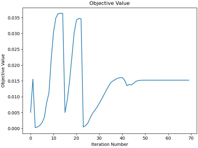
Plot the objective value.

_ = prob.plot_objective_value()

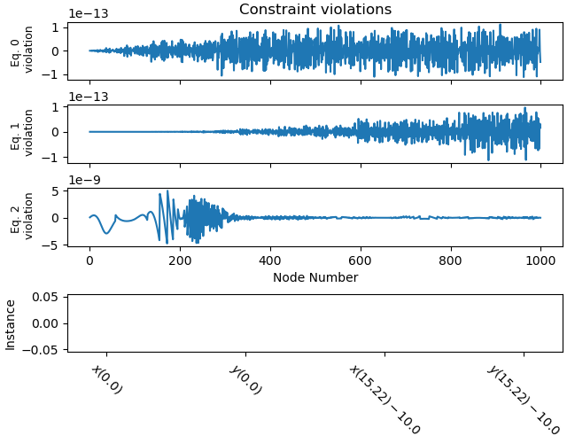
Plot the violations of the constraints.

_ = prob.plot_constraint_violations(solution, subplots=True)

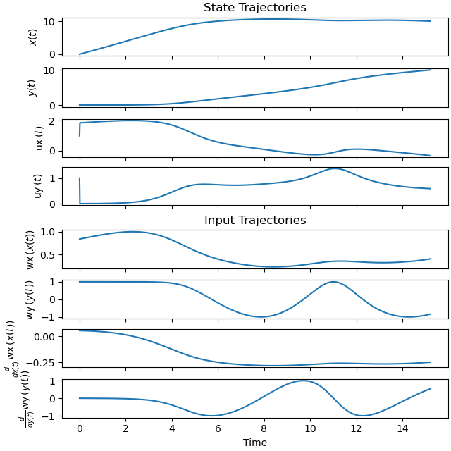
Plot the trajectories of the solution.

_ = prob.plot_trajectories(solution)

Animation.

fps = 5


def f(x, y):
    return speed_field_lam(x, y)


resultat, *_, h_val = prob.parse_free(solution)

x_min = np.min(resultat[0, :])
x_max = np.max(resultat[0, :])
y_min = np.min(resultat[1, :])
y_max = np.max(resultat[1, :])
x_max = max(x_max, y_max) + 1.0
x_min = min(x_min, y_min) - 1.0

t_arr = prob.time_vector(solution)
state_sol = CubicSpline(t_arr, resultat.T)

xx = np.linspace(x_min, x_max, 400)
yy = np.linspace(x_min, x_max, 400)
X, Y = np.meshgrid(xx, yy)
Z = f(X, Y)

fig, ax = plt.subplots(figsize=(8, 6), constrained_layout=True)
im = ax.pcolormesh(X, Y, Z, shading="auto", cmap="viridis")
fig.colorbar(im, ax=ax, label="speed [m/sec]")
ax.contour(X, Y, Z, levels=15, colors="white", linewidths=0.4, alpha=0.5)
ax.set_xlim(x_min, x_max)
ax.set_ylim(x_min, x_max)
ax.set_xlabel("x")
ax.set_ylabel("y")
ax.set_aspect("equal")

ax.scatter([0], [0], color="yellow", s=50, edgecolor="black", zorder=6)
ax.scatter([10], [10], color="green", s=50, zorder=6, edgecolor="black")

point, = ax.plot([], [], "o", color="red", mec="black", ms=11, zorder=5)
trail, = ax.plot([], [], "-", color="red", lw=2, zorder=4)

wp = (10.0, 10.0)
s = solutions[wp]
X, Y, _ = s.sol(np.linspace(0, 1, 500))
ax.plot(X, Y, lw=2, label=f"ray to {wp}", color="yellow")
ax.plot(*wp, "ko")
ax.plot([A[0], wp[0]], [A[1], wp[1]], "w--", lw=0.8)


def position(t):
    return state_sol(t)[:2]


T_var = travel_time(s)
delta_times = (h_val * (num_nodes - 1) - T_var) / T_var * 100
t_straight = straight_line_time([10.0, 10.0])


def update(t):
    px, py = position(t)
    point.set_data([px], [py])
    ts = np.linspace(0, t, 50)
    path = np.array([position(s) for s in ts])
    trail.set_data(path[:, 0], path[:, 1])

    msg = (f"Running time = {t:.3f} sec \n Lighter colors indicated "
           "higher speed "
           f"\n The yellow line is the solution of the variational problem \n"
           f"Travel time opty solution = {h_val * (num_nodes - 1):.3f} sec \n "
           f"Travel time variational solution = {T_var:.3f} sec \n"
           f"Along the straight line, travel time = {t_straight:.1f} sec"
           )

    ax.set_title(msg)
    return point, trail


frames = np.concatenate((np.arange(0, h_val * (num_nodes - 1), 1/fps),
                         [h_val * (num_nodes - 1)]))
ani = FuncAnimation(fig, update, frames=frames, interval=1000/fps,
                    blit=False, repeat=True)

plt.show()

Once Loop Reflect