Note
Go to the end to download the full example code.
Synchronisation of Clocks
Objectives
See, whether the observation first reported by Huygens in 1665 can be reproduced. See the article: https://physicsworld.com/a/the-secret-of-the-synchronized-pendulums/
Show how to use a smooth hump function to model a torque impulse applied to the pendulums.
Description
Two pendulums of length \(l_2\) and \(l_3\) are connected by a horizontal rod of length \(l_1\), which can move horizontally. The first pendulum is fixed at the left end of the horizontal rod, the second pendulum is fixed at the right end of the horizontal rod. The horizontal rod is connected to a \(O\) point by a spring and a damper. The first pendulum is connected to the horizontal rod by a spring and a damper of constants \(k_1\) and \(d_1\). The second pendulum is connected to the horizontal rod by a spring and a damper of constants \(k_2\) and \(d_2\).
Impulse torques of strength \(p_2\) and \(p_3\) are applied to the first and second pendulum, respectively. The impulse is modeled by a smooth hump function.
Notes
Only for certain combinations of the parameters was it possible to get the synchronisation effect. Maybe this is a reason, it is not observed all the time. I never found parameters, which would even remotely model two cuckoo clocks, hanging on a wall.
The torque impulses applied to the pendulums are modeled by a smooth hump, as numpy does not have a Dirac Delta function.
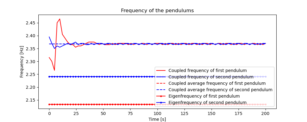
In the example. the common frequency is different from the eigenfrequency of the pendulums. Maybe this corresponds to the statement in the article, that the synchronized clocks will both show the wrong time.
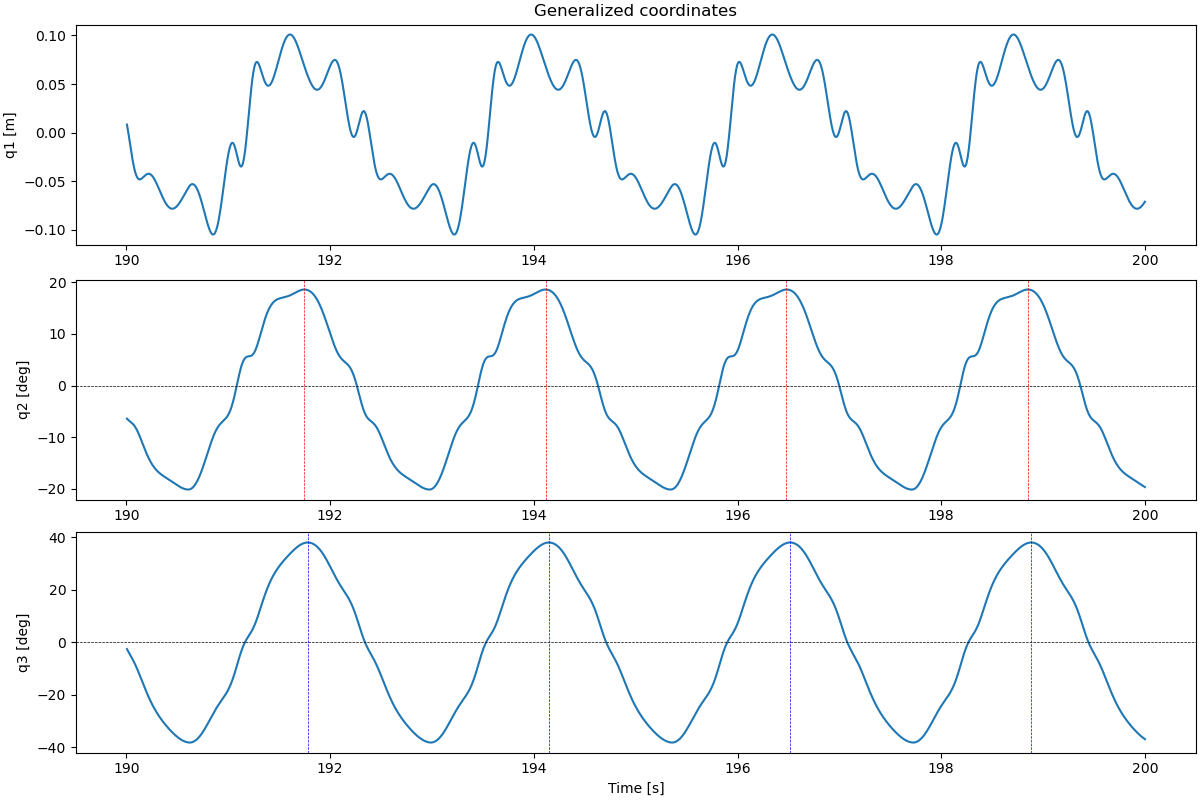
States
\(q_1\) : horizontal position of the horizontal rod
\(q_2\) : angle of the first pendulum
\(q_3\) : angle of the second pendulum
\(u_1\) : velocity of the horizontal rod
\(u_2\) : angular velocity of the first pendulum
\(u_3\) : angular velocity of the second pendulum
Parameters
\(m_1\) : mass of the horizontal rod
\(m_2\) : mass of the first pendulum
\(m_3\) : mass of the second pendulum
\(g\) : gravitational acceleration
\(l_1\) : length of the horizontal rod
\(l_2\) : length of the first pendulum
\(l_3\) : length of the second pendulum
\(k_1\) : spring constant of the horizontal rod
\(k_2\) : spring constant of the first pendulum
\(k_3\) : spring constant of the second pendulum
\(d_1\) : damping coefficient of the horizontal rod
\(d_2\) : damping coefficient of the first pendulum
\(d_3\) : damping coefficient of the second pendulum
\(p_2\) : impulse torque applied to the first pendulum
\(p_3\) : impulse torque applied to the second pendulum
import numpy as np
import sympy as sm
import sympy.physics.mechanics as me
from scipy.integrate import solve_ivp
from scipy.signal import find_peaks
import matplotlib.pyplot as plt
from scipy.interpolate import CubicSpline
from matplotlib.animation import FuncAnimation
Define a smooth hump function to model the impulse torque applied to the pendulums
def smooth_hump(x, a, b, steep):
return 0.5 * (1 - sm.tanh(steep * (x - a)) - sm.tanh(steep * (x - b)))
Equations of Motion
N, A1, A2, A3 = sm.symbols('N A1 A2 A3', cls=me.ReferenceFrame)
O, P1, P2, Dmc1, Dmc2, Dmc3 = sm.symbols('O P1 P2 Dmc1 Dmc2 Dmc3',
cls=me.Point)
O.set_vel(N, 0) # Set the velocity of the origin to zero
t = me.dynamicsymbols._t # Time symbol
q1, q2, q3, u1, u2, u3 = me.dynamicsymbols('q1 q2 q3 u1 u2 u3', real=True)
k1, k2, k3, m1, m2, m3 = sm.symbols('k1 k2 k3 m1 m2 m3')
d1, d2, d3 = sm.symbols('d1 d2 d3', real=True)
l1, l2, l3, g, p1, p2, p3 = sm.symbols('l1 l2 l3 g p1 p2 p3', real=True)
A1.orient_axis(N, 0, N.z)
A2.orient_axis(N, q2, N.z)
A3.orient_axis(N, q3, N.z)
A2.set_ang_vel(N, u2 * N.z)
A3.set_ang_vel(N, u3 * N.z)
Dmc1.set_pos(O, q1 * N.x)
Dmc1.set_vel(N, u1 * N.x)
P1.set_pos(Dmc1, -l1 / 2 * A1.x)
P1.v2pt_theory(Dmc1, N, A1)
P2.set_pos(Dmc1, l1 / 2 * A1.x)
P2.v2pt_theory(Dmc1, N, A1)
Dmc2.set_pos(P1, -l2 * A2.y)
Dmc2.v2pt_theory(P1, N, A2)
Dmc3.set_pos(P2, -l3 * A3.y)
Dmc3.v2pt_theory(P2, N, A3)
iZZ1 = 1 / 12 * m1 * l1**2
iZZ2 = 1 / 12 * m2 * l2**2
iZZ3 = 1 / 12 * m3 * l3**2
inert1 = me.inertia(A1, 0, 0, iZZ1)
inert2 = me.inertia(A2, 0, 0, iZZ2)
inert3 = me.inertia(A3, 0, 0, iZZ3)
# Create the bodies
body1 = me.RigidBody('body1', Dmc1, A1, m1, (inert1, Dmc1))
body2 = me.RigidBody('body2', Dmc2, A2, m2, (inert2, Dmc2))
body3 = me.RigidBody('body3', Dmc3, A3, m3, (inert3, Dmc3))
bodies = [body1, body2, body3]
# Create the forces
forces = [
(Dmc1, -m1 * g * N.y - k1 * q1 * N.x - d1 * u1 * N.x),
(Dmc2, -m2 * g * N.y),
(Dmc3, -m3 * g * N.y),
(A2, -k2 * q2 * A2.z - d2 * u2 * A2.z + p2 *
smooth_hump(q2, -0.01, 0.01, 25) * sm.sign(u2) * A2.z),
(A3, -k3 * q3 * A3.z - d3 * u3 * A3.z + p3 *
smooth_hump(q3, -0.01, 0.01, 25) * sm.sign(u3) * A3.z)
]
kd = sm.Matrix([u1 - q1.diff(t), u2 - q2.diff(t), u3 - q3.diff(t)])
q_ind = [q1, q2, q3]
u_ind = [u1, u2, u3]
KM = me.KanesMethod(N, q_ind=q_ind, u_ind=u_ind, kd_eqs=kd)
fr, frstar = KM.kanes_equations(bodies, forces)
force = KM.forcing_full
MM = KM.mass_matrix_full
sm.pprint(force)
⎡ u₁(t) ↪
⎢ ↪
⎢ u₂(t) ↪
⎢ ↪
⎢ u₃(t) ↪
⎢ ↪
⎢ 2 2 ↪
⎢ -d₁⋅u₁(t) - k₁⋅q₁(t) + l₂⋅m₂⋅u₂ (t)⋅sin(q₂(t)) + l₃⋅m₃⋅u₃ (t)⋅sin(q₃(t)) ↪
⎢ ↪
⎢-d₂⋅u₂(t) - g⋅l₂⋅m₂⋅sin(q₂(t)) - k₂⋅q₂(t) + p₂⋅(-0.5⋅tanh(25⋅q₂(t) - 0.25) - 0.5⋅tanh(25⋅q₂(t) + 0.25) + 0.5)⋅sign(u₂ ↪
⎢ ↪
⎣-d₃⋅u₃(t) - g⋅l₃⋅m₃⋅sin(q₃(t)) - k₃⋅q₃(t) + p₃⋅(-0.5⋅tanh(25⋅q₃(t) - 0.25) - 0.5⋅tanh(25⋅q₃(t) + 0.25) + 0.5)⋅sign(u₃ ↪
↪ ⎤
↪ ⎥
↪ ⎥
↪ ⎥
↪ ⎥
↪ ⎥
↪ ⎥
↪ ⎥
↪ ⎥
↪ (t))⎥
↪ ⎥
↪ (t))⎦
Lambdification
qL = [q1, q2, q3, u1, u2, u3]
pL = [m1, m2, m3, g, l1, l2, l3, k1, k2, k3, d1, d2, d3, p2, p3]
MM_lam = sm.lambdify(qL + pL, MM, cse=True)
force_lam = sm.lambdify(qL + pL, force, cse=True)
Numerical Integration
# Input variables
m21 = 1.0 # mass of the first vertical rod
m31 = 1.0 # mass of the second vertical rod
g1 = 9.81 # gravitational acceleration
l11 = 1.5 # length of the horizontal rod
l21 = 1.0 # length of the first vertical rod
l31 = 1.1 # length of the second vertical rod
k21 = 0.0 # spring constant of the first vertical rod
k31 = 0.0 # spring constant of the second vertical rod
d11 = 0.0 # damping coefficient of the horizontal rod
d21 = 0.2 # damping coefficient of the first vertical rod
d31 = 0.2 # damping coefficient of the second vertical rod
p21 = 0.45 # impulse torque applied to the first vertical rod
p31 = 0.475 # impulse torque applied to the second vertical rod
# Initial conditions
q11 = 0.0 # initial x position of the horizontal rod
q21 = np.deg2rad(30.0) # initial y position of the horizontal rod
q31 = np.deg2rad(30.0) # initial angle of the horizontal rod
u11 = 0.0
u21 = 0.0
u31 = 0.0
intervall = 200 # Simulation time in seconds
punkte = 200 # Evaluation points per second
schritte = int(intervall * punkte)
times = np.linspace(0., intervall, schritte)
t_span = (0., intervall)
max_step = 0.005 # Ensure solver does not miss the impulse.
def gradient(t, y, args):
sol = np.linalg.solve(MM_lam(*y, *args), force_lam(*y, *args))
return np.array(sol).T[0]
The second loop is to get the eigenfrequencies of the pendulums. The connecting mass is made very large, so the two pendulums swing (almost) independently.
frequenz2 = []
frequenz3 = []
peaks2 = []
peaks3 = []
min_values = []
resultat_list = []
for i in range(2):
if i == 0:
m11 = 0.01
k11 = 100.0
else:
m11 = 1.e10
k11 = 0.0
pL_vals = [m11, m21, m31, g1, l11, l21, l31, k11, k21, k31, d11, d21, d31,
p21, p31]
y0 = [q11, q21, q31, u11, u21, u31]
resultat1 = solve_ivp(gradient, t_span, y0, t_eval=times,
args=(pL_vals,), max_step=max_step)
resultat = resultat1.y.T
resultat_list.append(resultat)
print('resultat shape', resultat.shape)
print(resultat1.message)
print(f"the solve made {resultat1.nfev:,} function evaluations \n")
# Plotting the results
if i == 0:
anfang = int((intervall - 10.0) * punkte)
peak2, _ = find_peaks(resultat[anfang:, 1], height=np.deg2rad(10))
peak3, _ = find_peaks(resultat[anfang:, 2], height=np.deg2rad(20))
fig, ax = plt.subplots(3, 1, figsize=(12, 8), layout='constrained')
ax[0].plot(times[anfang:], resultat[anfang:, 0])
ax[1].plot(times[anfang:], np.rad2deg(resultat[anfang:, 1]))
ax[1].axhline(0.0, color='black', lw=0.5, ls='--')
for peak in peak2:
ax[1].axvline(times[anfang + peak], color='red', lw=0.5, ls='--')
ax[2].plot(times[anfang:], np.rad2deg(resultat[anfang:, 2]))
ax[2].axhline(0.0, color='black', lw=0.5, ls='--')
for peak in peak3:
ax[2].axvline(times[anfang + peak], color='blue', lw=0.5, ls='--')
ax[0].set_ylabel('q1 [m]')
ax[0].set_title('Generalized coordinates')
ax[1].set_ylabel('q2 [deg]')
ax[2].set_ylabel('q3 [deg]')
ax[2].set_xlabel('Time [s]')
peaks2_h, _ = find_peaks(resultat[200:, 1], height=np.deg2rad(10))
peaks3_h, _ = find_peaks(resultat[200:, 2], height=np.deg2rad(20))
frequenz2.append(np.array([peaks2_h[j + 1] - peaks2_h[j]
for j in range(len(peaks2_h) - 1)]))
frequenz3.append(np.array([peaks3_h[j + 1] - peaks3_h[j]
for j in range(len(peaks3_h) - 1)]))
min_values.append(min(len(frequenz2[i]), len(frequenz3[i])))
resultat shape (40000, 6)
The solver successfully reached the end of the integration interval.
the solve made 252,428 function evaluations
resultat shape (40000, 6)
The solver successfully reached the end of the integration interval.
the solve made 240,656 function evaluations
plot the frequencies of the pendulums.
eigenfrequency20 = np.mean(frequenz2[0]) / punkte
eigenfrequency30 = np.mean(frequenz3[0]) / punkte
eigenfrequency21 = np.mean(frequenz2[1]) / punkte
eigenfrequency31 = np.mean(frequenz3[1]) / punkte
min_value = min(min_values)
fig, ax = plt.subplots(1, 1, figsize=(10, 4))
ax.plot(np.linspace(0.0, intervall, min_value),
frequenz2[0][:min_value] / punkte, color='red',
label='Coupled frequency of first pendulum')
ax.plot(np.linspace(0.0, intervall, min_value),
frequenz3[0][:min_value] / punkte, color='blue',
label='Coupled frequency of second pendulum')
ax.plot(np.linspace(0.0, intervall, min_value),
np.ones(min_value) * eigenfrequency20, '--', color='red',
label='Coupled average frequency of first pendulum')
ax.plot(np.linspace(0.0, intervall, min_value),
np.ones(min_value) * eigenfrequency30, '--', color='blue',
label='Coupled average frequency of second pendulum')
ax.set_xlabel('Time [s]')
ax.set_ylabel('Frequency [Hz]')
ax.set_title('Frequency of the pendulums')
ax.plot(np.linspace(0.0, intervall, min_value),
np.ones(min_value) * eigenfrequency21, '.-', color='red',
label='Eigenfrequency of first pendulum')
ax.plot(np.linspace(0.0, intervall, min_value),
np.ones(min_value) * eigenfrequency31, '.-', color='blue',
label='Eigenfrequency of second pendulum')
_ = ax.legend()
Animate the Simulation
Only an excerpt of the total simulation is animated, as the the animation would take up too much memory otherwise Calculate the value of the maximum and minimum angles of the pendulums
peaks2, dicts2 = find_peaks(resultat_list[0][200:, 1], height=np.deg2rad(10))
trough2, dict_through2 = find_peaks(-resultat_list[0][200:, 1],
height=-np.deg2rad(10))
peaks3, dicts3 = find_peaks(resultat_list[0][200:, 2], height=np.deg2rad(20))
trough3, dict_through3 = find_peaks(-resultat_list[0][200:, 2],
height=-np.deg2rad(20))
peak2_average = np.mean(dicts2['peak_heights'])
print(f'Average height of peaks2: {np.rad2deg(peak2_average):.2f} deg')
peak3_average = np.mean(dicts3['peak_heights'])
print(f'Average height of peaks3: {np.rad2deg(peak3_average):.2f} deg')
trough2_average = -np.mean(dict_through2['peak_heights'])
print(f'Average height of troughs2: {np.rad2deg(trough2_average):.2f} deg')
trough3_average = -np.mean(dict_through3['peak_heights'])
print(f'Average height of troughs3: {np.rad2deg(trough3_average):.2f} deg')
fps = 8
t0, tf = 0.0, intervall
t_arr = np.linspace(t0, tf, schritte)
state_sol = CubicSpline(t_arr, resultat_list[0])
# Points at the end of the pendulums
P3, P4 = me.Point('P3'), me.Point('P4')
P3.set_pos(P1, -l2 * A2.y)
P4.set_pos(P2, -l3 * A3.y)
coordinates = P1.pos_from(O).to_matrix(N)
for point in [P2, P3, P4]:
coordinates = coordinates.row_join(point.pos_from(O).to_matrix(N))
coords_lam = sm.lambdify(qL + pL, coordinates, cse=True)
width, height, radius = 0.5, 0.5, 0.5
def init_plot():
xmin, xmax = -1.5, 2.0
ymin, ymax = -1.5, 0.5
fig, ax = plt.subplots(figsize=(8, 8))
ax.set_xlim(xmin, xmax)
ax.set_ylim(ymin, ymax)
ax.set_aspect('equal')
ax.set_xlabel('X-axis [m]')
ax.set_ylabel('Y-axis [m]')
line1, = ax.plot([], [], color='black', lw=1.0)
line2, = ax.plot([], [], color='red', lw=1.5)
line3, = ax.plot([], [], color='blue', lw=1.5)
line4 = ax.axvline(-0.5, color='red', lw=0.5, linestyle='--')
line5 = ax.axvline(0.5, color='red', lw=0.5, linestyle='--')
line6 = ax.axvline(0.0, color='blue', lw=0.5, linestyle='--')
line7 = ax.axvline(0.0, color='blue', lw=0.5, linestyle='--')
return fig, ax, point, line1, line2, line3, line4, line5, line6, line7
fig, ax, point, line1, line2, line3, line4, line5, line6, line7 = init_plot()
def update(t):
message = (f'Running time {t:0.2f} sec \n Speed 3 times actual speed \n '
f'The vertical dotted lines are the maximum \n average'
' deflections of the pendulums.')
ax.set_title(message)
coords = coords_lam(*state_sol(t), *pL_vals)
line1.set_data([coords[0, 0], coords[0, 1]], [coords[1, 0], coords[1, 1]])
line2.set_data([coords[0, 0], coords[0, 2]], [coords[1, 0], coords[1, 2]])
line3.set_data([coords[0, 1], coords[0, 3]], [coords[1, 1], coords[1, 3]])
line4.set_xdata([coords[0, 0] + l21 * np.sin(peak2_average),
coords[0, 0] + l21 * np.sin(peak2_average)])
line5.set_xdata([coords[0, 0] + l21 * np.sin(trough2_average),
coords[0, 0] + l21 * np.sin(trough2_average)])
line6.set_xdata([coords[0, 1] + l31 * np.sin(peak3_average),
coords[0, 1] + l31 * np.sin(peak3_average)])
line7.set_xdata([coords[0, 1] + l31 * np.sin(trough3_average),
coords[0, 1] + l31 * np.sin(trough3_average)])
# Create the animation.
anim = FuncAnimation(fig, update,
frames=np.arange(5, 45, 1/fps),
interval=1/fps*333.3)
plt.show()