Heat Diffusion Process with Inequality (betts_10_57)

This is example 10.57 from John T. Betts, Practical Methods for Optimal Control Using Nonlinear Programming, 3rd edition, chapter 10: Test Problems. It deals with the ‘discretization’ of a PDE.

More details may be found in section 6.2 of this book.

Notes

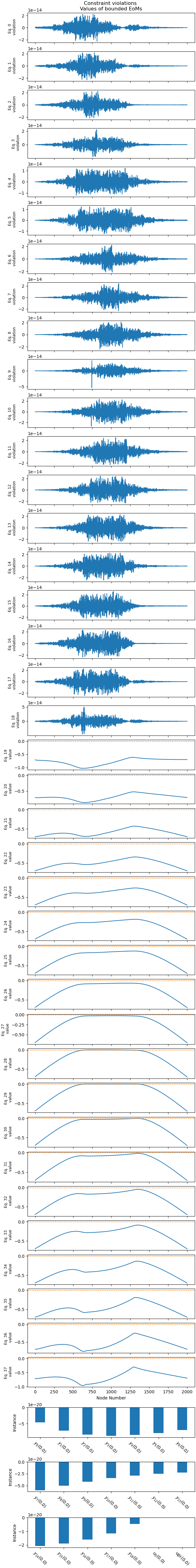
• The equations of motion consist of N - 1 differential quations and N - 1 algebraic equations. The latter are bound to be non - positive.

• As the time appears explicitly in the equations of motion, and currently opty does not support this, a function T(t) is defined and a known trajectory map is provided to opty.

States

• \(y_1, .....y_{N-1}\) : state variables

Specifieds

• \(u_0, u_{\ pi}\) : control variables

import numpy as np
import sympy as sm
import sympy.physics.mechanics as me
import time
from opty import Problem
from opty.utils import MathJaxRepr

Equations of motion.

t = me.dynamicsymbols._t
T = sm.symbols('T', cls=sm.Function)

N = 20

y = list(me.dynamicsymbols(f'y:{N-1}'))
u0, upi = me.dynamicsymbols('u0 upi')

# Parameters
q1 = 1.e-3
q2 = 1.e-3
a = 0.5
b = 0.2
c = 1.0
delta = sm.pi/N


def g(k, t):
    x = k * sm.pi/N
    return c * (sm.sin(x) * sm.sin(sm.pi*t/5) - a) - b


eom = sm.Matrix([
    -y[0].diff(t) + 1/delta**2 * (y[1] - 2*y[0] + u0),
    *[-y[i].diff(t) + 1/delta**2 * (y[i+1] - 2*y[i] + y[i-1])
      for i in range(1, N-2)],
    -y[N-2].diff(t) + 1/delta**2 * (upi - 2*y[N-2] + y[N-3]),
    *[g(k, T(t)) - y[k] for k in range(N-1)],
])

MathJaxRepr(eom)

$$\left[\begin{matrix}\frac{400 \left(u_{0} - 2 y_{0} + y_{1}\right)}{\pi^{2}} - \dot{y}_{0}\\\frac{400 \left(y_{0} - 2 y_{1} + y_{2}\right)}{\pi^{2}} - \dot{y}_{1}\\\frac{400 \left(y_{1} - 2 y_{2} + y_{3}\right)}{\pi^{2}} - \dot{y}_{2}\\\frac{400 \left(y_{2} - 2 y_{3} + y_{4}\right)}{\pi^{2}} - \dot{y}_{3}\\\frac{400 \left(y_{3} - 2 y_{4} + y_{5}\right)}{\pi^{2}} - \dot{y}_{4}\\\frac{400 \left(y_{4} - 2 y_{5} + y_{6}\right)}{\pi^{2}} - \dot{y}_{5}\\\frac{400 \left(y_{5} - 2 y_{6} + y_{7}\right)}{\pi^{2}} - \dot{y}_{6}\\\frac{400 \left(y_{6} - 2 y_{7} + y_{8}\right)}{\pi^{2}} - \dot{y}_{7}\\\frac{400 \left(y_{7} - 2 y_{8} + y_{9}\right)}{\pi^{2}} - \dot{y}_{8}\\\frac{400 \left(y_{10} + y_{8} - 2 y_{9}\right)}{\pi^{2}} - \dot{y}_{9}\\\frac{400 \left(- 2 y_{10} + y_{11} + y_{9}\right)}{\pi^{2}} - \dot{y}_{10}\\\frac{400 \left(y_{10} - 2 y_{11} + y_{12}\right)}{\pi^{2}} - \dot{y}_{11}\\\frac{400 \left(y_{11} - 2 y_{12} + y_{13}\right)}{\pi^{2}} - \dot{y}_{12}\\\frac{400 \left(y_{12} - 2 y_{13} + y_{14}\right)}{\pi^{2}} - \dot{y}_{13}\\\frac{400 \left(y_{13} - 2 y_{14} + y_{15}\right)}{\pi^{2}} - \dot{y}_{14}\\\frac{400 \left(y_{14} - 2 y_{15} + y_{16}\right)}{\pi^{2}} - \dot{y}_{15}\\\frac{400 \left(y_{15} - 2 y_{16} + y_{17}\right)}{\pi^{2}} - \dot{y}_{16}\\\frac{400 \left(y_{16} - 2 y_{17} + y_{18}\right)}{\pi^{2}} - \dot{y}_{17}\\\frac{400 \left(upi + y_{17} - 2 y_{18}\right)}{\pi^{2}} - \dot{y}_{18}\\- y_{0} - 0.7\\- y_{1} + 1.0 \left(- \frac{\sqrt{2} \sqrt{\frac{5}{8} - \frac{\sqrt{5}}{8}}}{2} + \frac{\sqrt{2} \left(\frac{1}{4} + \frac{\sqrt{5}}{4}\right)}{2}\right) \sin{\left(\frac{\pi T}{5} \right)} - 0.7\\- y_{2} + 1.0 \left(- \frac{1}{4} + \frac{\sqrt{5}}{4}\right) \sin{\left(\frac{\pi T}{5} \right)} - 0.7\\- y_{3} + 1.0 \left(\frac{\sqrt{2} \left(\frac{1}{4} - \frac{\sqrt{5}}{4}\right)}{2} + \frac{\sqrt{2} \sqrt{\frac{\sqrt{5}}{8} + \frac{5}{8}}}{2}\right) \sin{\left(\frac{\pi T}{5} \right)} - 0.7\\- y_{4} + 1.0 \sqrt{\frac{5}{8} - \frac{\sqrt{5}}{8}} \sin{\left(\frac{\pi T}{5} \right)} - 0.7\\- y_{5} + 0.5 \sqrt{2} \sin{\left(\frac{\pi T}{5} \right)} - 0.7\\- y_{6} + 1.0 \left(\frac{1}{4} + \frac{\sqrt{5}}{4}\right) \sin{\left(\frac{\pi T}{5} \right)} - 0.7\\- y_{7} + 1.0 \left(- \frac{\sqrt{2} \left(\frac{1}{4} - \frac{\sqrt{5}}{4}\right)}{2} + \frac{\sqrt{2} \sqrt{\frac{\sqrt{5}}{8} + \frac{5}{8}}}{2}\right) \sin{\left(\frac{\pi T}{5} \right)} - 0.7\\- y_{8} + 1.0 \sqrt{\frac{\sqrt{5}}{8} + \frac{5}{8}} \sin{\left(\frac{\pi T}{5} \right)} - 0.7\\- y_{9} + 1.0 \left(\frac{\sqrt{2} \sqrt{\frac{5}{8} - \frac{\sqrt{5}}{8}}}{2} + \frac{\sqrt{2} \left(\frac{1}{4} + \frac{\sqrt{5}}{4}\right)}{2}\right) \sin{\left(\frac{\pi T}{5} \right)} - 0.7\\- y_{10} + 1.0 \sin{\left(\frac{\pi T}{5} \right)} - 0.7\\- y_{11} + 1.0 \left(\frac{\sqrt{2} \sqrt{\frac{5}{8} - \frac{\sqrt{5}}{8}}}{2} + \frac{\sqrt{2} \left(\frac{1}{4} + \frac{\sqrt{5}}{4}\right)}{2}\right) \sin{\left(\frac{\pi T}{5} \right)} - 0.7\\- y_{12} + 1.0 \sqrt{\frac{\sqrt{5}}{8} + \frac{5}{8}} \sin{\left(\frac{\pi T}{5} \right)} - 0.7\\- y_{13} + 1.0 \left(- \frac{\sqrt{2} \left(\frac{1}{4} - \frac{\sqrt{5}}{4}\right)}{2} + \frac{\sqrt{2} \sqrt{\frac{\sqrt{5}}{8} + \frac{5}{8}}}{2}\right) \sin{\left(\frac{\pi T}{5} \right)} - 0.7\\- y_{14} + 1.0 \left(\frac{1}{4} + \frac{\sqrt{5}}{4}\right) \sin{\left(\frac{\pi T}{5} \right)} - 0.7\\- y_{15} + 0.5 \sqrt{2} \sin{\left(\frac{\pi T}{5} \right)} - 0.7\\- y_{16} + 1.0 \sqrt{\frac{5}{8} - \frac{\sqrt{5}}{8}} \sin{\left(\frac{\pi T}{5} \right)} - 0.7\\- y_{17} + 1.0 \left(\frac{\sqrt{2} \left(\frac{1}{4} - \frac{\sqrt{5}}{4}\right)}{2} + \frac{\sqrt{2} \sqrt{\frac{\sqrt{5}}{8} + \frac{5}{8}}}{2}\right) \sin{\left(\frac{\pi T}{5} \right)} - 0.7\\- y_{18} + 1.0 \left(- \frac{1}{4} + \frac{\sqrt{5}}{4}\right) \sin{\left(\frac{\pi T}{5} \right)} - 0.7\end{matrix}\right]$$

Set Up and Solve the Optimization Problem

t0, tf = 0.0, 5.0
num_nodes = 2001
interval_value = (tf - t0) / (num_nodes - 1)

state_symbols = y
specified_symbols = (u0, upi)

times = np.linspace(t0, tf, num=num_nodes)

Specify the objective function and form the gradient.

def obj(free):
    value1 = interval_value * ((delta/2 + q1) *
                               np.sum(free[N*num_nodes:(N+1)*num_nodes]**2))
    value2 = interval_value * ((delta/2 + q2) *
                               np.sum(free[(N+1)*num_nodes:
                                           (N+2)*num_nodes]**2))
    value3 = delta * interval_value * np.sum(free[0:N*num_nodes]**2)
    return value1 + value2 + value3


def obj_grad(free):
    grad = np.zeros_like(free)
    grad[N*num_nodes:(N+1)*num_nodes] = \
        (2 * (delta/2 + q1) * interval_value *
         free[N*num_nodes:(N+1)*num_nodes])
    grad[(N+1)*num_nodes:(N+2)*num_nodes] = \
        (2 * (delta/2 + q2) * interval_value *
         free[(N+1)*num_nodes:(N+2)*num_nodes])
    grad[0:N*num_nodes] = (2 * delta * interval_value * free[0:N*num_nodes])
    return grad

Specify the instance constraints

instance_constraints = (
    *[y[i].func(t0) for i in range(N-1)],
    u0.func(t0),
    upi.func(t0),
)

Inequality bounds on the last 19 eoms.

eom_bounds = {k: (-np.inf, 0.0) for k in range(N-1, 2*N-2)}

Create the optimization problem.

prob = Problem(
    obj,
    obj_grad,
    eom,
    state_symbols,
    num_nodes,
    interval_value,
    instance_constraints=instance_constraints,
    known_trajectory_map={T(t): times},
    eom_bounds=eom_bounds,
)

Give some rough estimates for the trajectories.

initial_guess = np.zeros(prob.num_free)

Find the optimal solution.

for _ in range(1):
    start = time.time()
    solution, info = prob.solve(initial_guess)
    initial_guess = solution
    print(info['status_msg'])
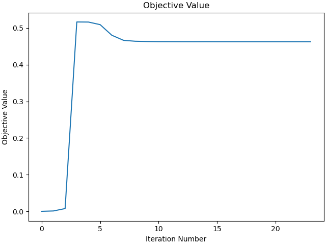
    Jstar = 0.468159793
    print(f"Objective value achieved: {info['obj_val']:.4f}, as per the book "
          f"it is {Jstar:.4f}, so the error is: "
          f"{(info['obj_val'] - Jstar) / (Jstar)*100:.3f} % ")
    print(f'Time taken for the simulation: {time.time() - start:.2f} s')

b'Algorithm terminated successfully at a locally optimal point, satisfying the convergence tolerances (can be specified by options).'
Objective value achieved: 0.4627, as per the book it is 0.4682, so the error is: -1.163 %
Time taken for the simulation: 143.32 s

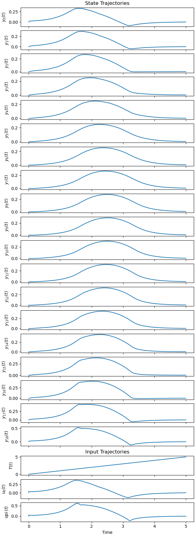
Plot the optimal state and input trajectories.

_ = prob.plot_trajectories(solution)

Plot the constraint violations.

_ = prob.plot_constraint_violations(solution, subplots=True, show_bounds=True)

Plot the objective function.

_ = prob.plot_objective_value()