Note
Go to the end to download the full example code.
Closed Chain
Objective
Show that sympy.physics.mechanics can handle systems consisting of a large number of bodies
Description
A chain is simulated as a closed 2D n-link pendulum, where each link is modelled as a rod. The two ends of the chain are fixed at \((0., 0.)\) and at \((EP_x, EP_y)\).
Notes
I saw this some time ago as an example of some other modeling library, and I wanted to see, how this would work with sympy.physics.mechanics.
If the rotation of frame \(A_i\) is defined relative to frame \(A_{i-1}\) the number of operations shoot up: for n = 12 the mass matrix has 25 mio operations. If the rotation of \(A_i\) is defined relative to the inertial frame \(O\), the numbers become very reasonable.
The catenary is the shape of a chain of uniform linear density hanging under the influence of gravity only. This will be drawn in the animation. If there is friction, the chain should approach this catenary shape.
Variables and Parameters
\(O\) : Inertial frame, fixed in place
\(PO\) : Point fixed in \(O\), where the chain is suspended
\(A_i\) : Body fixed frame of link \(i\), with \(0 \leq i < n\)
\(Dmc_i\) : Center of gravity of link \(i\)
\(P_i\) : Point, where frame \(A_i\) joins frame \(A_{i+1}\)
\(l\) : Length of the pendulum, that is each link has length \(\dfrac{l}{n}\)
\(m\) : Mass of each link
\(iZZ\) : Moment of inertial of each link around \(A_i.z\), relative to \(Dmc_i\)
\(\textrm{reibung}\) : Speed dependent friction in each joint.
\(aux_x, aux_y, f_x, f_y\) : virtual speeds and reaction forces on point \(O\)
\(rhs\) : ‘place holders’ for the \(rhs = MM^{-1} \cdot force\) to be evaluated numerically later
\(q_i\) : Generalized coordinate of frame \(A_i\) relative to the inertial frame \(O\).
\(u_i\) : Angular speed of frame \(A_i\) relative to the inertial frame \(O\).
\(EP\) : End point of the chain, fixed in place. That is \(P[n-1]\) should be at \(EP\).
\(EP_x, EP_y\) : Its coordinates
import sympy as sm
import sympy.physics.mechanics as me
import numpy as np
from scipy.integrate import solve_ivp
from scipy.optimize import fsolve, minimize, root
import matplotlib.pyplot as plt
from matplotlib import animation
Kanes Equations
Set up the geometry. n is the number of links in the chain.
n = 60
term_info = False
m, g, iZZ, l, reibung = sm.symbols('m, g, iZZ, l, reibung')
q = me.dynamicsymbols(f'q:{n}')
u = me.dynamicsymbols(f'u:{n}')
auxx, auxy, fx, fy = me.dynamicsymbols('auxx, auxy, fx, fy')
t = me.dynamicsymbols._t
A = sm.symbols(f'A:{n}', cls=me.ReferenceFrame)
Dmc = sm.symbols(f'Dmc:{n}', cls=me.Point)
P = sm.symbols(f'P:{n}', cls=me.Point)
rhs = list(sm.symbols(f'rhs:{n}'))
O = me.ReferenceFrame('O')
PO = me.Point('PO')
PO.set_vel(O, auxx*O.x + auxy*O.y)
l1 = l/n
l2 = l/(2 * n)
A[0].orient_axis(O, q[0], O.z)
A[0].set_ang_vel(O, u[0] * O.z)
Dmc[0].set_pos(PO, l2*A[0].x)
Dmc[0].v2pt_theory(PO, O, A[0])
P[0].set_pos(PO, l1*A[0].x)
P[0].v2pt_theory(PO, O, A[0])
for i in range(1, n):
A[i].orient_axis(O, q[i], O.z)
A[i].set_ang_vel(O, u[i] * O.z)
Dmc[i].set_pos(P[i-1], l2*A[i].x)
Dmc[i].v2pt_theory(P[i-1], O, A[i])
P[i].set_pos(P[i-1], l1*A[i].x)
P[i].v2pt_theory(P[i-1], O, A[i])
Set the configuration constraint and derive the speed constraints from it.
The last point \(P[n-1]\) is required to be fixed at \((EP_x / EP_y)\). laenge is used to check how well the speed constraints are fulfilled. .magnitude() runs into numerical issues sometimes. This was discussed on Github a while ago. This way avoids these issues.
EP = me.Point('EP')
EPx, EPy = sm.symbols('EPx, EPy')
EP_pos = EP.set_pos(PO, EPx*O.x + EPy*O.y)
EP_pos = EP.pos_from(PO)
Pn_pos = P[0].pos_from(PO) + sum([P[i+1].pos_from(P[i]) for i in range(n-1)])
constraint = EP_pos - Pn_pos
constraintX = me.dot(constraint, O.x)
constraintY = me.dot(constraint, O.y)
constraint_matrix = sm.Matrix([constraintX, constraintY])
# using magnitude() here gives errors at times.
laenge = sm.sqrt(constraintX**2 + constraintY**2)
# Velocity constraints
constraint_dict = {sm.Derivative(q[i], t): u[i] for i in range(n)}
constraintXdt = constraintX.diff(t).subs(constraint_dict)
constraintYdt = constraintY.diff(t).subs(constraint_dict)
constraintdt_matrix = sm.Matrix([constraintXdt, constraintYdt])
# Solve for the dependent speeds :math:`u[n-2], u[n-1]`, needed for the
# initial conditions for solve_ivp below
matrix_A = constraintdt_matrix.jacobian((u[n-2], u[n-1]))
vector_b = constraintdt_matrix.subs({u[n-2]: 0., u[n-1]: 0.})
loesung = matrix_A.LUsolve(-vector_b)
if term_info is True:
print('loesung DS', me.find_dynamicsymbols(loesung))
print('loesung FS', loesung.free_symbols)
print(f'loesung has {sm.count_ops(loesung):,} operations')
constraint_matrix = [constraint_matrix[0, 0], constraint_matrix[1, 0]]
constraintdt_matrix = [constraintdt_matrix[0, 0], constraintdt_matrix[1, 0]]
loesung has 2,025 operations
Kane’s Equations
BODY = []
for i in range(n):
inertia = me.inertia(A[i], 0., 0., iZZ)
body = me.RigidBody('body' + str(i), Dmc[i], A[i], m, (inertia, Dmc[i]))
BODY.append(body)
FL1 = [(Dmc[i], -m*g*O.y) for i in range(n)] + [(PO, fx*O.x + fy*O.y)]
Torque = [(A[i], - u[i] * reibung * A[i].z) for i in range(n)]
FL = FL1 + Torque
kd = [u[i] - q[i].diff(t) for i in range(n)]
aux = [auxx, auxy]
speed_constr = [u[n-2] - loesung[0], u[n-1] - loesung[1]]
u_ind = [u[i] for i in range(n-2)]
u_dep = [u[n-2], u[n-1]]
KM = me.KanesMethod(
O,
q_ind=q,
u_ind=u_ind,
u_dependent=u_dep,
kd_eqs=kd,
u_auxiliary=aux,
velocity_constraints=speed_constr,
)
fr, frstar = KM.kanes_equations(BODY, FL)
MM = KM.mass_matrix_full
if term_info is True:
print('MM DS', me.find_dynamicsymbols(MM))
print('MM free symbols', MM.free_symbols)
print(f'MM contains {sm.count_ops(MM):,} operations')
force = KM.forcing_full.subs({fx: 0., fy: 0.})
if term_info is True:
print('force DS', me.find_dynamicsymbols(force))
print('force free symbols', force.free_symbols)
print(f'force contains {sm.count_ops(force):,} operations')
# This is needed for the reaction forces on the suspension point PO.
eingepraegt_dict = {sm.Derivative(i, t): j for i, j in zip(u, rhs)}
eingepraegt = KM.auxiliary_eqs.subs(eingepraegt_dict)
if term_info is True:
print('eingepraegt DS', me.find_dynamicsymbols(eingepraegt))
print('eingepraegt free symbols', eingepraegt.free_symbols)
print(f'eingepraegt has {sm.count_ops(eingepraegt):,} operations')
MM contains 423,204 operations
force contains 230,764 operations
eingepraegt has 2,149 operations
Functions for the kinetic and the potential energies. Always useful to detect mistakes. orte is needed for the animation only.
kin_energie = sum([koerper.kinetic_energy(O)
for koerper in BODY]).subs({i: 0. for i in aux})
pot_energie = sum([m*g*me.dot(koerper.pos_from(PO), O.y) for koerper in Dmc])
orte = [[me.dot(P[i].pos_from(PO), uv) for uv in (O.x, O.y)] for i in range(n)]
Lambdification.
qL = q + u_ind + u_dep
qL1 = q + u_ind
qL2 = [q[i] for i in range(n-2)]
pL = [m, g, l, iZZ, reibung, EPx, EPy]
F = [fx, fy]
MM_lam = sm.lambdify(qL + pL, MM, cse=True)
force_lam = sm.lambdify(qL + pL, force, cse=True)
eingepraegt_lam = sm.lambdify(F + qL + pL + rhs, eingepraegt, cse=True)
kin_lam = sm.lambdify(qL + pL, kin_energie, cse=True)
pot_lam = sm.lambdify(qL + pL, pot_energie, cse=True)
ort_lam = sm.lambdify(qL + pL, orte, cse=True)
loesung_lam = sm.lambdify(qL1 + pL, loesung, cse=True)
constraint_lam = sm.lambdify([q[n-2], q[n-1]] + qL2 + pL, constraint_matrix,
cse=True)
laenge_lam = sm.lambdify(q + pL, laenge, cse=True)
constraintdt_lam = sm.lambdify(qL + pL, constraintdt_matrix, cse=True)
Numerical Integration
A.
Define the initial values and the parameters.
For more than a few links, it is difficult to get initial generalized coordinates \(q[i]\) which fit the configuration constraint: if \(q[0]....q[n-3]\) are set randomly, there may not be a solution for the dependent generalized coordinates \(q[n-2], q[n-1]\). So get approximate generalized coordinates by numerically solving \(\min \limits_{q[0]...q[n-1]} (| \textrm{config. constraint} |)\) for \(q[0]....q[n-1]\). method = ‘Nelder-Meat’ in minimize(..) finds good minimal values even for larger n, while no method even failed with n = 10, depending on where the fixed point of \(P[n-1]\) was located. There are many feasible solutions, the one picked likely depends on the initial conditions given to minimize(..). The values produced by minimize(..) serve as ininital conditions to numerically solve for \(q[n-2], q[n-1]\) Finally it calculates how well the initial generalized coordinates and speeds fulfill the configuaration constraint and the resulting speed constraints.
# Input variables
m1 = 1.
g1 = 9.8
l1 = 30.
reibung1 = 5.0
q1 = [np.random.choice((1, -1)) for _ in range(n)] # starting guess for below.
# setting the angular velocities != 0 ,increases the integration time a lot.
u1 = [0. for _ in range(n)]
EPx1 = 10. # Must be > 0, else the catenary will not work.
EPy1 = 3.
intervall = 20.
punkte = 25
schritte = int(intervall * punkte)
times = np.linspace(0., intervall, schritte)
t_span = (0., intervall)
iZZ1 = 1./12. * m1 * (l1/n)**2 # from the internet
pL_vals = [m1, g1, l1, iZZ1, reibung1, EPx1, EPy1]
if np.sqrt(EPx1**2 + EPy1**2) > l1:
raise Exception('endpoint to far away from (0/0)')
find generalized coordinates to fullfill the configuration constraints
def func1(x0, args):
return laenge_lam(*x0, *args)
X0 = tuple((q1))
X0 = tuple(([1.] * n))
for _ in range(6):
t0 = minimize(func1, X0, pL_vals, method='Nelder-Mead')
X0 = t0.x
print((f'error of initial guess is {laenge_lam(*X0, *pL_vals):.3e}'
f', achieved by minimizing'))
error of initial guess is 6.830e-11, achieved by minimizing
Use the approximate generalized coordinates to find the dependent generalized coordinates.
def func2(X0, args):
return constraint_lam(*X0, *args)
args = [X0[i] for i in range(n-2)] + pL_vals
Z0 = (X0[n-2], X0[n-1])
for _ in range(6):
t0 = fsolve(func2, Z0, args)
Z0 = t0
Q0 = [Z0[0], Z0[1]] + [X0[i] for i in range(n-2)]
print((f'error of improved guess is {laenge_lam(*Q0, *pL_vals):.3e}'
f' achieved by numerically solve for the dependent coordinates. \n'))
# find the dependent speeds to match the independet speeds
U0 = [u1[i] for i in range(n-2)]
t0 = loesung_lam(*Q0, *U0, *pL_vals)
u1[n-2] = t0[0][0]
u1[n-1] = t0[1][0]
y0 = Q0 + U0 + [u1[n-2], u1[n-1]]
print((f'error in the initial speed constraints are X: '
f'{constraintdt_lam(*y0, *pL_vals)[0]:.3e} '
f'Y: {constraintdt_lam(*y0, *pL_vals)[1]:.3e}'))
error of improved guess is 2.011e-15 achieved by numerically solve for the dependent coordinates.
error in the initial speed constraints are X: 0.000e+00 Y: 0.000e+00
B.
Numerical integration. method = \(\textrm{Radau}\) seems to keep the total energy closer to constant, absent any friction, that is \(\textrm{reibung}_1 = 0\).
y0 = Q0 + U0 + [u1[n-2], u1[n-1]]
def gradient(t, y, args):
sol = np.linalg.solve(MM_lam(*y, *args), force_lam(*y, *args))
return np.array(sol).T[0]
resultat1 = solve_ivp(gradient, t_span, y0, t_eval=times, args=(pL_vals,),
method='Radau', atol=1.e-5, rtol=1.e-5)
resultat = resultat1.y.T
print('resultat shape', resultat.shape, '\n')
print(resultat1.message, '\n')
print((f"To numerically integrate an intervall of {intervall:.2f} sec "
f"the routine made {resultat1.nfev:,} function calls."))
resultat shape (500, 120)
The solver successfully reached the end of the integration interval.
To numerically integrate an intervall of 20.00 sec the routine made 5,558 function calls.
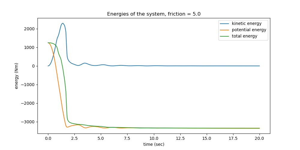
Plot the energies.
kin_np = np.empty(schritte)
pot_np = np.empty(schritte)
total_np = np.empty(schritte)
for i in range(schritte):
pot_np[i] = pot_lam(*[resultat[i, j] for j in range(resultat.shape[1])],
*pL_vals)
kin_np[i] = kin_lam(*[resultat[i, j] for j in range(resultat.shape[1])],
*pL_vals)
total_np[i] = kin_np[i] + pot_np[i]
if reibung1 == 0.:
max_total = np.max(np.abs(total_np))
min_total = np.min(np.abs(total_np))
delta = max_total - min_total
print((f'max deviation of total energy from zero is '
f'{delta/max_total * 100:.3e} % of max. total energy'))
fig, ax = plt.subplots(figsize=(10, 5))
for i, j in zip((kin_np, pot_np, total_np), ('kinetic energy',
'potential energy',
'total energy')):
ax.plot(times, i, label=j)
ax.set_title(f'Energies of the system, friction = {reibung1}')
ax.set_xlabel('time (sec)')
ax.set_ylabel('energy (Nm)')
_ = ax.legend()
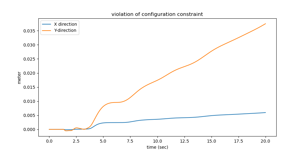
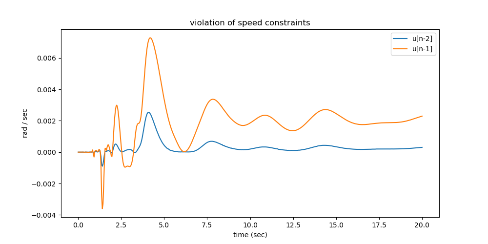
Check, how well the configuration constraint and the speed constraints are kept. Ideally, of course, they should be zero.
X_np = np.empty(schritte)
Y_np = np.empty(schritte)
for i in range(schritte):
X_np[i], Y_np[i] = constraint_lam(resultat[i, n-2], resultat[i, n-1],
*[resultat[i, j] for j in range(n-2)],
*pL_vals)
fig, ax = plt.subplots(figsize=(10, 5))
for i, j in zip((X_np, Y_np), ('X direction', 'Y-direction')):
ax.plot(times, i, label=j)
ax.set_title('violation of configuration constraint')
ax.set_xlabel('time (sec)')
ax.set_ylabel('meter')
_ = ax.legend()
for i in range(schritte):
X_np[i], Y_np[i] = constraintdt_lam(*[resultat[i, j] for j in
range(resultat.shape[1])], *pL_vals)
fig, ax = plt.subplots(figsize=(10, 5))
for i, j in zip((X_np, Y_np), ('u[n-2]', 'u[n-1]')):
ax.plot(times, i, label=j)
ax.set_title('violation of speed constraints')
ax.set_xlabel('time (sec)')
ax.set_ylabel('rad / sec')
_ = ax.legend()
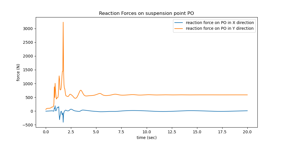
Reaction force on \(P_O\)
First solve the equation \(rhs = MM^{-1} \cdot force\) numerically. Then solve \(\textrm{eingepraegt} = 0\) for \(fx, fy\) numerically.
resultat2 = resultat
schritte2 = schritte
times2 = times
RHS1 = np.empty((schritte2, resultat2.shape[1]))
for i in range(schritte2):
RHS1[i, :] = np.linalg.solve(MM_lam(*[resultat2[i, j]
for j in range(resultat2.shape[1])],
*pL_vals),
force_lam(*[resultat2[i, j]
for j in range(resultat2.shape[1])],
*pL_vals)).reshape(resultat2.shape[1])
print('RHS1 shape', RHS1.shape)
# calculate implied forces numerically
def func(x, *args):
# serves to 'modify' the arguments for root.
return eingepraegt_lam(*x, *args).reshape(2)
for _ in range(2):
kraftx = np.empty(schritte2)
krafty = np.empty(schritte2)
x0 = tuple((1., 1.)) # initial guess
for i in range(schritte2):
for _ in range(2):
y0 = [resultat2[i, j] for j in range(resultat2.shape[1])]
rhs = [RHS1[i, j] for j in range(n, 2*n)]
args = tuple(y0 + pL_vals + rhs)
AAA = root(func, x0, args=args)
AAA = AAA.x
x0 = tuple(AAA)
kraftx[i] = AAA[0]
krafty[i] = AAA[1]
fig, ax = plt.subplots(figsize=(10, 5))
for i, j in zip((kraftx, krafty), ('reaction force on PO in X direction',
'reaction force on PO in Y direction',
'reaction force on P[n-1] in X direction')):
plt.plot(times2, i, label=j)
ax.set_title('Reaction Forces on suspension point PO')
ax.set_xlabel('time (sec)')
ax.set_ylabel('force (N)')
_ = plt.legend()
RHS1 shape (500, 120)
Catenary
The shape of a chain of uniform linear density hanging symmetric to the vertical Y axis is described by \(y(x) = factor \cdot \cosh(\dfrac{x}{factor})\) A chain suspended at \((x_1, y_1)\) and \((x_2, y_2)\) and length \(l\) where
\(v = y_2 - y_1\)
\(h = x_2 - x_1\)
\(l\): length of the chain
has this transcendental equation for factor:
\(\sqrt{l^2 - v^2} = 2 \cdot factor \cdot \sinh(\dfrac{h}{2. \cdot factor})\)
Numerically solve this equation for factor, called t0 in the program. factor is inserted in the equation for the suspended chain, to get the graph of a symmetrically hanging chain. Next calculate the value of delta, called \(d_0\) in the program, where the chain is at \(EP_y\). Then appropriately shift this symmetric chain so it matches the chain simulated If friction is used, that is \(\textrm{reibung}_1 > 0\), the chain should approach this catenary.
It seems that if the catenary becomes ‘extreme’ in some way, the equation to solve for factor does not converge well. The longer the chain, the better the result seems to be.
Iteration from \(EP_y = 0\), where it always seems to calculate correctly, to \(EP_y\).
faktor, xx, yy, delta = sm.symbols('faktor, xx, yy, delta')
catenary = 2. * faktor * sm.sinh(EPx / (2. * faktor)) - sm.sqrt(l**2 - EPy**2)
catenary_lam = sm.lambdify([faktor, EPx, EPy, l], catenary, cse=True)
def func3(X0, args):
return catenary_lam(*X0, *args)
catenaryY = faktor * sm.cosh((xx)/(faktor))
catenaryY_lam = sm.lambdify([xx, faktor, EPx], catenaryY, cse=True)
catenaryZ = faktor * sm.cosh((xx + delta)/(faktor))
catenaryZ_lam = sm.lambdify([delta, xx, faktor], catenaryZ, cse=True)
def func4(X0):
return catenaryZ_lam(X0, EPx1/2., t0) - catenaryZ_lam(0.,
-EPx1/2, t0) - EPy2
Delta = []
Factor = []
zahl = 20
EPy2 = 0.
X01 = 0.1
z01 = 0.1
delta = EPy1/zahl
for _ in range(zahl):
EPy2 += delta
args = [EPx1, EPy2, l1]
t0 = fsolve(func3, X01, args)
t0 = t0[0]
X01 = t0
Factor.append(t0)
d0 = fsolve(func4, z01)
z01 = d0[0]
Delta.append(z01)
# calculate the values of the catenary to be used below in the animation
ergebnis = []
for xx1 in np.linspace(0., EPx1, 100):
ergebnis.append(catenaryY_lam(xx1-(EPx1-d0)/2., t0, EPx1))
abzug = ergebnis[0]
for i in range(100):
ergebnis[i] = ergebnis[i] - abzug
Animation
# get Carthesian coordinates
x_coords = np.empty((len(times), n+1))
y_coords = np.empty((len(times), n+1))
for j in range(schritte):
x_coords[j] = [0.] + [ort_lam(*[resultat[j, k]
for k in range(resultat.shape[1])],
*pL_vals)[k11][0]
for k11 in range(n)]
y_coords[j] = [0.] + [ort_lam(*[resultat[j, k]
for k in range(resultat.shape[1])],
*pL_vals)[k11][1]
for k11 in range(n)]
max_x = max([abs(x_coords[i, j])for i in range(schritte) for j in range(n+1)])
max_y = max([abs(y_coords[i, j])for i in range(schritte) for j in range(n+1)])
max_xy = max(max_x, max_y)
fig, ax = plt.subplots(figsize=(7, 7))
ax.axis('on')
ax.set(xlim=(-max_xy-1., max_xy+1.), ylim=(-max_xy-1., max_xy+1.))
ax.plot(0., 0.4, marker='v', markersize=15, color='red')
ax.plot(EPx1, EPy1 + 0.4, marker='v', markersize=15, color='red')
ax.plot(np.linspace(0., EPx1*1.01, 100), ergebnis, color='red', lw=0.3)
# Connects the poinbts.
line, = ax.plot([], [], 'o-', lw=0.5, color='blue', markersize=0)
def animate_pendulum(times, x, y):
def animate(i):
ax.set_title((f'Running time is {i / schritte * intervall:.2f} sec \n'
f'The red curve is the catenary'), fontsize=12)
line.set_data(x[i], y[i])
return line,
anim = animation.FuncAnimation(fig, animate, frames=len(times),
interval=1000*times.max() / len(times),
blit=True)
return anim
anim = animate_pendulum(times, x_coords, y_coords)
plt.show()