Note
Go to the end to download the full example code.
Rolling Axle, Controlled
Description
This is a modification of the rolling axle on an uneven street example, see
https://pydy.org/pst-notebooks/examples/plot_rolling_axle_uneven_street.html
There, with the no slip conditions enforced, the system has only one degree of freedom, so controlling it to reach some fixed point is not possible.
Now, I want it to move to some final position by applying torques to the
wheels. Hence the no slip conditions are relaxed, using opnty’s
eom_bounds keyword.
Notes
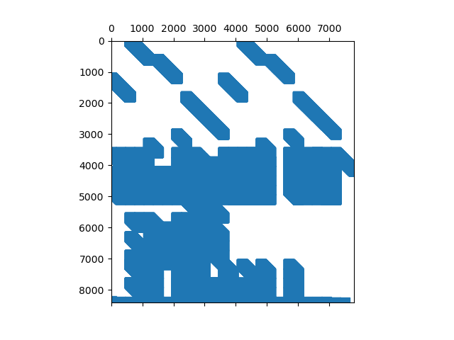
It takes quite long to get an acceptable solution, presumably because the jacobian is not very sparse.
I am not very sure about the ‘mechanical meaning’ of the relaxed no slip conditions.
The animation is a bit ‘jumpy’ to save space. It may be improved by using a larger value for
fps.
States
\(q_L, q_R\) : rotation angles of the wheels
\(x_L, y_L\) : coordinates of the contact point of the left wheel
\(q_2, q_3\) : rotation angles of the axle
\(x_R, y_R\) : coordinates of the contact point of the right wheel
\(l_y, l_z\) : components of the vector from the contact point to the center of the left wheel
\(r_y, r_z\) : components of the vector from the contact point to the center of the right wheel
\(u_L, u_R\) : angular speeds of the wheels
\(u_2, u_3\) : angular speeds of the axle
\(ux_L, uy_L\) : speeds of the contact point of the left wheel
\(ux_R, uy_R\) : speeds of the contact point of the right wheel
\(ul_y, ul_z\) : speeds of the vector from the contact point to the center of the left wheel
\(ur_y, ur_z\) : speeds of the vector from the contact point to the center of the right wheel
\(T_L, T_R\) : torques applied to the wheels. Controls of opty
Parameters
\(m_L, m_R\) : masses of the wheels
\(m_o\) : mass of the particle attached to the wheels
\(g\) : gravity
\(r_L, r_R\) : radii of the wheels
\(l\) : distance between the wheels
\(amplitude, frequenz\) : parameters of the street
\(reibung\) : friction between the wheels and the axle
Further symbols
\(N\) : inertial frame
\(AX\) : frame attached to the axle
\(AL\) : frame attached to the left wheel
\(AR\) : frame attached to the right wheel
\(O\) : reference point, fixed in N
\(CPL\) : contact point of the left wheel
\(CPR\) : contact point of the right wheel
\(Dmc_L\) : center of mass of the left wheel
\(Dmc_R\) : center of mass of the right wheel
\(m_{Dmc_L}\) : particle attached to the left wheel
\(m_{Dmc_R}\) : particle attached to the right wheel
import sympy as sm
import sympy.physics.mechanics as me
import numpy as np
import matplotlib.pyplot as plt
from scipy.interpolate import interp1d
from scipy.optimize import root, minimize
from opty import Problem
from matplotlib.animation import FuncAnimation
from matplotlib.patches import Ellipse
from matplotlib.transforms import Affine2D
If True, print some information about the eom.
info = True
Rotation angles of the wheels and the body, and their speeds.
qL, qR, q2, q3 = me.dynamicsymbols('qL qR q2 q3')
uL, uR, u2, u3 = me.dynamicsymbols('uL uR u2 u3')
Coordinates of the contact points of the left / right wheel.
xL, yL, xR, yR = me.dynamicsymbols('xL yL xR yR')
uxL, uyL, uxR, uyR = me.dynamicsymbols('uxL uyL uxR uyR') # their 'speeds'
Components of the vectors from the contact points to the centers of mass, in N. Their speeds.
ly, lz, ry, rz = me.dynamicsymbols('ly lz ry rz')
uly, ulz, ury, urz = me.dynamicsymbols('uly ulz ury urz')
Torques on the wheels. Controls for opty.
TL, TR = me.dynamicsymbols('TL TR')
Parameters of the system: masses, gravity, radii of the wheels, and distance between the wheels.
mL, mR, mo, g, rL, rR, l = sm.symbols(
'mL mR mo g rL rR l')
Parameters for the surface.
amplitude, frequenz, reibung = sm.symbols('amplitude frequenz reibung')
Define some frames, points, etc.
N, AX, AL, AR = sm.symbols('N, AX, AL, AR', cls=me.ReferenceFrame)
O, CPL, CPR, DmcL, DmcR = sm.symbols('O, CPL, CPR, DmcL, DmcR',
cls=me.Point)
m_DmcL, m_DmcR = sm.symbols('m_DmcL, m_DmcR', cls=me.Point)
O.set_vel(N, 0)
t = me.dynamicsymbols._t
The axle does not rotate around itself.
AX.orient_body_fixed(N, [q3, q2, 0], 'ZYX')
rot = AX.ang_vel_in(N)
AX.set_ang_vel(N, u2*AX.y + u3*AX.z)
rot1 = AX.ang_vel_in(N)
The left wheel rotates around the axle, that is, around AX.x, similarly for the right wheel.
AL.orient_axis(AX, qL, AX.x)
AL.set_ang_vel(AX, uL*AX.x)
AR.orient_axis(AX, qR, AX.x)
AR.set_ang_vel(AX, uR*AX.x)
Particles attached to the wheels.
m_DmcL.set_pos(DmcL, rL*AL.y)
m_DmcR.set_pos(DmcR, rR*AR.y)
Here the street is modelled. rumpel must be an integer.
x_h, y_h = sm.symbols('x_h y_h')
rumpel = 2
def gesamt(x, y, amplitude, frequenz, rumpel):
strasse = sum([amplitude/j * (sm.sin(j*frequenz*sm.pi * x) +
sm.sin(j*frequenz*sm.pi * y))
for j in range(1, rumpel)])
return strasse
def gesamt_plot(x_h, y_h, amplitude, frequenz):
return sum([amplitude/j * (sm.sin(j*frequenz*sm.pi * x_h) +
sm.sin(j*frequenz*sm.pi * y_h))
for j in range(1, rumpel)])
Create the dictionary to replace \(\dfrac{d}{dt}(\textrm{gen. coord})\) with the corresponding symbols.
kin_dict = {
xL.diff(t): uxL,
yL.diff(t): uyL,
xR.diff(t): uxR,
yR.diff(t): uyR,
qL.diff(t): uL,
qR.diff(t): uR,
ly.diff(t): uly,
lz.diff(t): ulz,
ry.diff(t): ury,
rz.diff(t): urz,
q2.diff(t): u2,
q3.diff(t): u3,
}
kin_dict
{Derivative(xL(t), t): uxL(t), Derivative(yL(t), t): uyL(t), Derivative(xR(t), t): uxR(t), Derivative(yR(t), t): uyR(t), Derivative(qL(t), t): uL(t), Derivative(qR(t), t): uR(t), Derivative(ly(t), t): uly(t), Derivative(lz(t), t): ulz(t), Derivative(ry(t), t): ury(t), Derivative(rz(t), t): urz(t), Derivative(q2(t), t): u2(t), Derivative(q3(t), t): u3(t)}
Configuration Constraints
\(CP_L, CP_R\) are the contact points where the wheels touch the street.
CPL.set_pos(O, xL*N.x + yL*N.y +
gesamt(xL, yL, amplitude, frequenz, rumpel)*N.z)
CPL.set_vel(N, uxL * N.x + uyL * N.y +
gesamt(xL, yL, amplitude, frequenz, rumpel).diff(t) * N.z)
Define the vectors pointing from the contact point to the corresponding center of the wheel. \(\text{vector}_L \perp A.x\) and \(\text{vector}_R \perp A.x\), so they have no component in A.x direction.
vectorL = ly * AX.y + lz * AX.z
vectorR = ry * AX.y + rz * AX.z
\(\text{vector}_L\) and \(\text{vector}_R\) must have magnitude equal to the respective wheel \(r_L\) and \(r_R\).
constr_length = sm.Matrix([
vectorL.magnitude() - rL,
vectorR.magnitude() - rR,
])
constr_length
Matrix([
[-rL + sqrt(ly(t)**2 + lz(t)**2)],
[-rR + sqrt(ry(t)**2 + rz(t)**2)]])
Set centers of mass of wheels, second contact point CPR.
DmcL.set_pos(CPL, vectorL)
DmcL.v2pt_theory(CPL, N, AX)
DmcR.set_pos(DmcL, l * AX.x)
CPR.set_pos(DmcR, -vectorR)
\(\text{vector}_L\) must be in the plane formed by the gradient \(n_L\) at the point (xL, yL) on the surface and by \(A.x\) the direction of the axle, that is \(\text{vector}_L \circ (n_L \times A.x) = 0\) Same for \(\text{vector}_R\).
nL = (-gesamt(xL, yL, amplitude, frequenz, rumpel).diff(xL) * N.x -
gesamt(xL, yL, amplitude, frequenz, rumpel).diff(yL) * N.y +
N.z).normalize()
nR = (-gesamt(xR, yR, amplitude, frequenz, rumpel).diff(xR) * N.x -
gesamt(xR, yR, amplitude, frequenz, rumpel).diff(yR) * N.y +
N.z).normalize()
perpL = nL.cross(AX.x)
perpR = nR.cross(AX.x)
constrT = sm.Matrix([
perpL.dot(vectorL),
perpR.dot(vectorR),
])
Determine the constraints for \(x_R, y_R, q_2\) for the location of CPR.
CPR_pos = xR*N.x + yR*N.y + gesamt(xR, yR, amplitude, frequenz, rumpel)*N.z
delta_loc = CPR.pos_from(O) - CPR_pos
constr_CPR = sm.Matrix([
delta_loc.dot(N.x),
delta_loc.dot(N.y),
delta_loc.dot(N.z),
])
Combine the configuration constraints.
config_constr = constr_length.col_join(constrT).col_join(constr_CPR)
if info:
print(f"config_constr contains {sm.count_ops(config_constr)} operations")
print("DS", me.find_dynamicsymbols(config_constr))
print("FS", config_constr.free_symbols, "shape = ", config_constr.shape)
config_constr contains 484 operations
DS {ly(t), xL(t), yR(t), q3(t), lz(t), q2(t), ry(t), xR(t), yL(t), rz(t)}
FS {l, rR, frequenz, t, rL, amplitude} shape = (7, 1)
No Slip Constraints
Set the speeds of the centers of the wheels and of the particles attached to it.
DmcL.v2pt_theory(CPL, N, AL)
DmcR.v2pt_theory(CPR, N, AR)
vDmcL = DmcL.pos_from(O).diff(t, N)
vDmcR = DmcR.pos_from(O).diff(t, N)
deltaL_vel = vDmcL - DmcL.vel(N)
deltaR_vel = vDmcR - DmcR.vel(N)
frame = N
constr_no_slip = sm.Matrix([
deltaL_vel.dot(frame.x),
deltaL_vel.dot(frame.y),
deltaR_vel.dot(frame.x),
deltaR_vel.dot(frame.y),
])
m_DmcL.v2pt_theory(DmcL, N, AL)
_ = m_DmcR.v2pt_theory(DmcR, N, AR)
Kane’s Equations
iXXL = 0.5 * mL * rL**2
iYYL = 0.25 * mL * rL**2
iZZL = 0.25 * mL * rL**2
iXXR = 0.5 * mR * rR**2
iYYR = 0.25 * mR * rR**2
iZZR = 0.25 * mR * rR**2
IL = me.inertia(AL, iXXL, iYYL, iZZL)
IR = me.inertia(AR, iXXR, iYYR, iZZR)
BodyL = me.RigidBody('BodyL', DmcL, AL, mL, (IL, DmcL))
BodyR = me.RigidBody('BodyR', DmcR, AR, mR, (IR, DmcR))
partL = me.Particle('partL', m_DmcL, mo)
partR = me.Particle('partR', m_DmcR, mo)
BODY = [BodyL, BodyR, partL, partR]
Set the external forces acting on the system.
FL1 = [(DmcL, -mL*g*N.z), (DmcR, -mR*g*N.z),
(m_DmcL, -mo*g*N.z), (m_DmcR, -mo*g*N.z)]
Torque = [(AL, -reibung * uL*AX.x), (AR, -reibung * uR*AX.x)]
The control for opty.
TorqueC = [(AL, TL*AL.x), (AR, TR*AR.x)]
Combine the forces and torques.
FL = FL1 + Torque + TorqueC
Kane’s method.
speed_constr = config_constr.diff(t)
kd = sm.Matrix([key - value for key, value in kin_dict.items()])
q_ind = [qL, qR, xL, yL, q3]
q_dep = [xR, yR, q2, ly, lz, ry, rz]
u_ind = [uL, uR, uxL, uyL, u3]
u_dep = [uxR, uyR, u2, uly, ulz, ury, urz]
kane = me.KanesMethod(
N,
q_ind=q_ind,
q_dependent=q_dep,
u_ind=u_ind,
u_dependent=u_dep,
kd_eqs=kd,
velocity_constraints=speed_constr,
configuration_constraints=config_constr,
)
fr, frstar = kane.kanes_equations(BODY, FL)
eom1 = kd.col_join(fr + frstar)
Append the configuration constraints.
eom2 = eom1.col_join(config_constr)
Append the non-slip constraints. They will be loosened in the optimization problem.
eom = eom2.col_join(constr_no_slip)
# Print some information about the eom.
if info:
print(f"eom have {sm.count_ops(eom):,} operations, "
f"{sm.count_ops(sm.cse(eom)):,} after cse, "
f"shape = {eom.shape}, \n")
print("eom dynamic symbols", me.find_dynamicsymbols(eom))
print("shapes of eom", eom.shape)
eom have 2,035,388 operations, 1,868 after cse, shape = (28, 1),
eom dynamic symbols {Derivative(uxL(t), t), uyL(t), Derivative(qL(t), t), Derivative(q3(t), t), Derivative(uyL(t), t), Derivative(rz(t), t), Derivative(yR(t), t), qR(t), uL(t), Derivative(ry(t), t), uR(t), rz(t), ulz(t), xL(t), TL(t), Derivative(q2(t), t), q2(t), Derivative(uL(t), t), u3(t), urz(t), yL(t), ry(t), Derivative(xR(t), t), Derivative(uR(t), t), ly(t), yR(t), Derivative(u2(t), t), uxL(t), Derivative(yL(t), t), q3(t), lz(t), TR(t), Derivative(ly(t), t), u2(t), xR(t), Derivative(lz(t), t), uly(t), Derivative(qR(t), t), Derivative(ury(t), t), Derivative(xL(t), t), Derivative(urz(t), t), uyR(t), qL(t), ury(t), uxR(t), Derivative(u3(t), t)}
shapes of eom (28, 1)
Set parameters.
par_map = {}
par_map[mL] = 1.0
par_map[mR] = 0.25
par_map[mo] = 0.1
par_map[g] = 9.81
par_map[rL] = 2.0
par_map[rR] = 1.0
par_map[l] = 5.0
par_map[amplitude] = 0.15
par_map[frequenz] = 0.25
par_map[reibung] = 1.0
Set the independent gen. coordinates.
qL1 = 0.0
qR1 = 0.0
xL1 = 1.0
yL1 = 0.0
q31 = 0.0
Final position of the contact point of the left wheel.
xL_end = 20.0
yL_end = 20.0
Calculate consistent initial dependent generalized coordinates. All generalized speeds are set to zero initially.
pL = [key for key in par_map.keys()]
pL_vals = [par_map[key] for key in pL]
config_constr_lam = sm.lambdify(q_dep + q_ind + pL, config_constr, cse=True)
def func(y, args):
return config_constr_lam(*y, *args).squeeze()
y0 = np.zeros(len(q_dep))
args = [qL1, qR1, xL1, yL1, q31] + pL_vals
res = root(func, y0, args=args)
xR1, yR1, q21, ly1, lz1, ry1, rz1 = res.x
if res.x[4] <= 0 or res.x[6] <= 0:
raise ValueError(f"use different initial guess, lz = {res.x[4]}, "
f"rz = {res.x[6]} meaning at least one wheel is "
"below the street")
for i, j in zip(q_dep, res.x):
print(f"{i} = {j:.3f}")
xR(t) = 6.090
yR(t) = -0.126
q2(t) = 0.249
ly(t) = -0.246
lz(t) = 1.985
ry(t) = -0.120
rz(t) = 0.993
Set up Problem
h = sm.symbols('h')
num_nodes = 300
t0, tf = 0.0, h * (num_nodes - 1)
interval_value = h
state_symbols = q_ind + q_dep + u_ind + u_dep
instance_constraints = [
qL.func(t0) - qL1,
qR.func(t0) - qR1,
xL.func(t0) - xL1,
yL.func(t0) - yL1,
q3.func(t0) - q31,
xR.func(t0) - xR1,
yR.func(t0) - yR1,
q2.func(t0) - q21,
ly.func(t0) - ly1,
lz.func(t0) - lz1,
ry.func(t0) - ry1,
rz.func(t0) - rz1,
*[speed.func(t0) - 0.0 for speed in u_ind + u_dep],
TL.func(t0) - 0.0,
TR.func(t0) - 0.0,
xL.func(tf) - xL_end,
yL.func(tf) - yL_end,
*[speed.func(tf) - 0.0 for speed in u_ind + u_dep],
]
def obj(free):
# Minimize the duration.
return free[-1]
def obj_grad(free):
grad = np.zeros_like(free)
grad[-1] = 1.0
return grad
limit = 50.0
bounds = {
h: (0.0, 0.1),
TL: (-limit, limit),
TR: (-limit, limit),
lz: (0.0, par_map[rL]), # left hub must remain above the street
rz: (0.0, par_map[rR]), # right hub must remain above the street
}
Loosen the non slip constraints.
delta_eom = 7.5 # Arbitrary. Not sure about the mechanical meaning.
eom_bounds = {
24: (-delta_eom, delta_eom),
25: (-delta_eom, delta_eom),
26: (-delta_eom, delta_eom),
27: (-delta_eom, delta_eom),
}
prob = Problem(
obj,
obj_grad,
eom,
state_symbols,
num_nodes,
h,
known_parameter_map=par_map,
instance_constraints=instance_constraints,
time_symbol=t,
bounds=bounds,
eom_bounds=eom_bounds,
)
Solve the Problem
initial_guess = np.ones(prob.num_free)
initial_guess[-1] = 0.005
for i in range(3):
if i == 0:
prob.add_option('max_iter', 50)
elif i == 1:
prob.add_option('max_iter', 1000)
else:
prob.add_option('max_iter', 25000)
solution, info = prob.solve(initial_guess)
print(info['status_msg'])
initial_guess = solution
b'Maximum number of iterations exceeded (can be specified by an option).'
b'Maximum number of iterations exceeded (can be specified by an option).'
b'Algorithm terminated successfully at a locally optimal point, satisfying the convergence tolerances (can be specified by options).'
Plot the constraint violations.
_ = prob.plot_constraint_violations(solution, subplots=True, show_bounds=True)

Plot the trajectories.
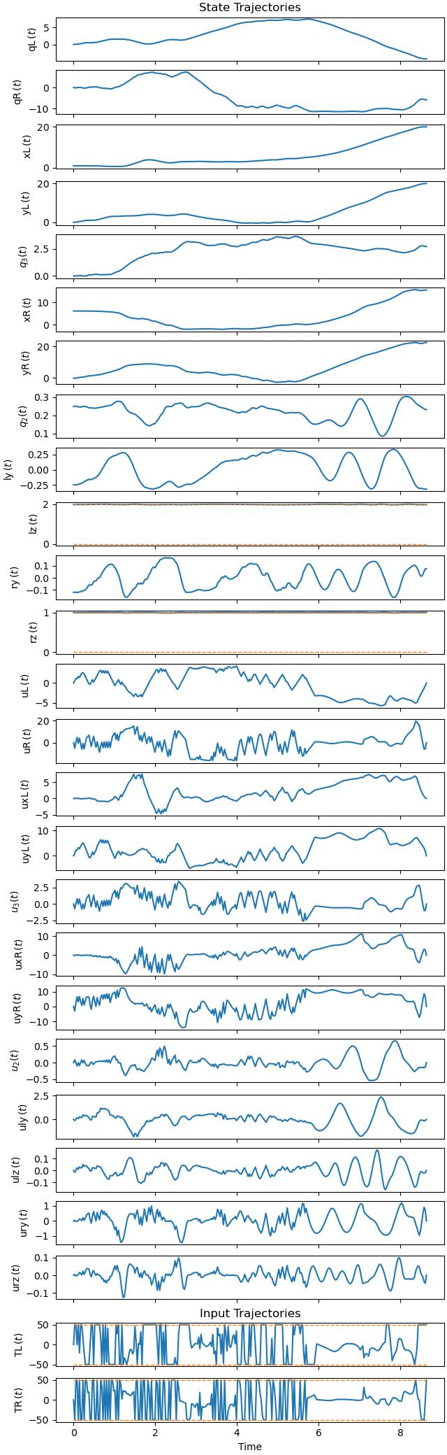
_ = prob.plot_trajectories(solution, show_bounds=True)
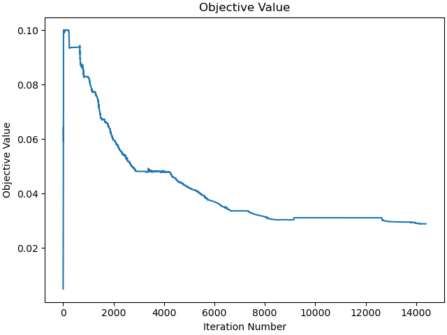
Plot the objective value over iterations.
_ = prob.plot_objective_value()
Plot the sparsity pattern of the Jacobian.
_ = prob.plot_jacobian_sparsity()
Find the minimum curvature of the surface and check it is larger than the wheels. (Formula from the internet)
x_h, y_h = sm.symbols('x_h y_h')
fx = gesamt_plot(x_h, y_h, amplitude, frequenz).diff(x_h)
fy = gesamt_plot(x_h, y_h, amplitude, frequenz).diff(y_h)
fxx = gesamt_plot(x_h, y_h, amplitude, frequenz).diff(x_h, 2)
fyy = gesamt_plot(x_h, y_h, amplitude, frequenz).diff(y_h, 2)
fxy = gesamt_plot(x_h, y_h, amplitude, frequenz).diff(x_h, y_h)
E = 1 + fx**2
F = fx * fy
G = 1 + fy**2
L = fxx / sm.sqrt(1 + fx**2 + fy**2)
M = fxy / sm.sqrt(1 + fx**2 + fy**2)
NN = fyy / sm.sqrt(1 + fx**2 + fy**2)
I1 = sm.Matrix([[E, F],
[F, G]])
II = sm.Matrix([[L, M],
[M, NN]])
# Shape operator
S = I1.inv() * II
# Eigenvalues = principal curvatures
k1, k2 = S.eigenvals().keys()
k1_lam = sm.lambdify([x_h, y_h, amplitude, frequenz], k1, cse=True)
k2_lam = sm.lambdify([x_h, y_h, amplitude, frequenz], k2, cse=True)
def func1(x0, args):
# just needed to get the arguments matching for minimuze
return np.abs(1.0 / k1_lam(*x0, *args))
def func2(x0, args):
# just needed to get the arguments matching for minimuze
return np.abs(1.0 / k2_lam(*x0, *args))
x0 = np.array((5.0, 10.0)) # initial guess
args = np.array((par_map[amplitude], par_map[frequenz]))
for _ in range(10):
minimal1 = minimize(func1, x0, args, tol=1e-6)
x0 = minimal1.x
for _ in range(10):
minimal2 = minimize(func2, x0, args, tol=1e-6)
x0 = minimal2.x
print("minimal1:", minimal1.message)
print("minimal2:", minimal2.message)
min_radius = min(minimal1.fun, minimal2.fun)
print('maximally admissible radius = {:.4f}'.format(min_radius))
if min_radius < max(par_map[rL], par_map[rR]):
raise ValueError("The initial conditions are not viable, because "
"the radius of the wheels is larger than the maximally "
"admissible radius.")
minimal1: Optimization terminated successfully.
minimal2: Optimization terminated successfully.
maximally admissible radius = 10.8076
Distance between \(Dmc_L\) and \(Dmc_R\) should be constant. Distance of \(CP_L\), \(CP_R\) from the surface of the street should be zero.
resultat, *_, h_act = prob.parse_free(solution)
resultat = resultat.T
sys_times = np.linspace(t0, num_nodes * h_act, num_nodes)
delta_CPL_z = CPL.pos_from(O).dot(N.z) - gesamt(xL, yL, amplitude, frequenz,
rumpel)
delta_CPL_z = me.msubs(delta_CPL_z, kin_dict)
delta_CPL_z_lam = sm.lambdify(q_ind + q_dep + u_ind + u_dep + pL, delta_CPL_z,
cse=True)
delta_CPR_z = CPR.pos_from(O).dot(N.z) - gesamt(xR, yR, amplitude, frequenz,
rumpel)
delta_CPR_z = me.msubs(delta_CPR_z, kin_dict)
delta_CPR_z_lam = sm.lambdify(q_ind + q_dep + u_ind + u_dep + pL, delta_CPR_z,
cse=True)
Dmc_dist = DmcL.pos_from(DmcR).magnitude()
Dmc_dist = me.msubs(Dmc_dist, kin_dict)
Dmc_dist_lam = sm.lambdify(q_ind + q_dep + u_ind + u_dep + pL, Dmc_dist,
cse=True)
dist_np = np.empty(resultat.shape[0])
CPL_z_np = np.empty(resultat.shape[0])
CPR_z_np = np.empty(resultat.shape[0])
for i in range(resultat.shape[0]):
CPL_z_np[i] = delta_CPL_z_lam(*[resultat[i, j] for j in range(24)],
*pL_vals)
CPR_z_np[i] = delta_CPR_z_lam(*[resultat[i, j] for j in range(24)],
*pL_vals)
dist_np[i] = Dmc_dist_lam(*[resultat[i, j] for j in range(24)],
*pL_vals)
fig, ax = plt.subplots(1, 1, figsize=(10, 3))
ax.plot(sys_times[0: resultat.shape[0]], dist_np,
label='distance between centers of mass')
ax.plot(sys_times[0: resultat.shape[0]], CPL_z_np,
label='CPL z coordinate')
ax.plot(sys_times[0: resultat.shape[0]], CPR_z_np,
label='CPR z coordinate')
ax.legend(loc='upper left')
ax.set_title('Distance between centers of mass and '
'z coordinates of CPL and CPR')
ax.set_xlabel('Time [s]')
ax.set_ylabel('Distance [m]')
max_dist = np.max(dist_np)
min_dist = np.min(dist_np)
print("Error in distance between centers of mass from being constant: "
f"{(max_dist - min_dist) / min_dist:.4e}")
print(F"error in CPL z coordinate from being equal to the road height: "
f"{(np.max(CPL_z_np) - np.min(CPL_z_np)):.4e}")
print(F"error in CPR z coordinate from being equal to the road height: "
f"{(np.max(CPR_z_np) - np.min(CPR_z_np)):.4e}")
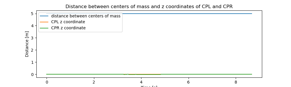
Error in distance between centers of mass from being constant: 0.0000e+00
error in CPL z coordinate from being equal to the road height: 0.0000e+00
error in CPR z coordinate from being equal to the road height: 2.1768e-11
Animation
fps = 7
rL1 = par_map[rL]
rR1 = par_map[rR]
amplitude1 = par_map[amplitude]
frequenz1 = par_map[frequenz]
resultat, *_, h_act = prob.parse_free(solution)
resultat = resultat.T
print(f"actual time step h = {h_act:.4f}")
t_arr = np.linspace(t0, num_nodes*h_act, num_nodes)
state_sol = interp1d(t_arr, resultat, kind='cubic', axis=0)
coordinates = DmcL.pos_from(O).to_matrix(N)
for point in (DmcR, m_DmcL, m_DmcR):
coordinates = coordinates.row_join(point.pos_from(O).to_matrix(N))
coords_lam = sm.lambdify(state_symbols + pL, coordinates, cse=True)
max_x = np.max(np.concatenate((resultat[:, 2], resultat[:, 5])))
max_y = np.max(np.concatenate((resultat[:, 3], resultat[:, 6])))
min_x = np.min(np.concatenate((resultat[:, 2], resultat[:, 5])))
min_y = np.min(np.concatenate((resultat[:, 3], resultat[:, 6])))
gesamt_plot_lam = sm.lambdify([x_h, y_h, amplitude, frequenz],
gesamt_plot(x_h, y_h, amplitude, frequenz),
cse=True)
max_radius = 2.0 * max(rL1, rR1)
xx = np.linspace(min_x-max_radius, max_x+max_radius, 100)
yy = np.linspace(min_y-max_radius, max_y+max_radius, 100)
XX, YY = np.meshgrid(xx, yy)
ZZ = gesamt_plot_lam(XX, YY, amplitude1, frequenz1)
fig, ax = plt.subplots(figsize=(7, 7))
ax.set_xlim(min_x-max_radius, max_x+max_radius)
ax.set_ylim(min_y-max_radius, max_y+max_radius)
ax.set_aspect('equal')
ax.set_xlabel('x', fontsize=15)
ax.set_ylabel('y', fontsize=15)
cf = ax.contourf(XX, YY, ZZ, levels=50, cmap='viridis')
fig.colorbar(cf, label='z value [m]', shrink=0.8)
# axle
line1, = ax.plot([], [], lw=1, marker='o', markersize=0, color='red')
# particles attached to the wheels
line4 = ax.scatter([], [], color='black', s=20)
line5 = ax.scatter([], [], color='black', s=20)
# startpoint, endpoint
ax.scatter([xL1], [yL1], color='red', s=50, edgecolor='black')
ax.scatter([xL_end], [yL_end], color='green', s=50, edgecolor='black')
# ellipses defined in local frame AX
winkel_q2 = state_sol(0)[7]
ellipseL = Ellipse((0, 0), width=2.0*rL1*np.sin(winkel_q2),
height=2.0*rL1,
fill=True, lw=2, color='red', alpha=0.5)
ax.add_patch(ellipseL)
ellipseR = Ellipse((0, 0), width=2.0*rR1*np.sin(winkel_q2),
height=2.0*rR1,
fill=True, lw=2, color='magenta', alpha=0.5)
ax.add_patch(ellipseR)
def update(t):
message = (f'Running time {t:.2f} sec. \n'
f'The left wheel is red with radius {rL1}, the '
f'right wheel is magenta \n with radius {rR1}.'
f' The black dots are the particles attached \n to the wheels')
ax.set_title(message, fontsize=11)
coords = coords_lam(*state_sol(t), *pL_vals)
line1.set_data([coords[0, 0], coords[0, 1]], [coords[1, 0], coords[1, 1]])
line4.set_offsets([coords[0, 2], coords[1, 2]])
line5.set_offsets([coords[0, 3], coords[1, 3]])
# transform from AX → inertial frame
theta = state_sol(t)[4]
X = coords[0, 0]
Y = coords[1, 0]
transform = Affine2D().rotate(theta).translate(X, Y) + ax.transData
ellipseL.set_width(2.0*rL1*np.sin(state_sol(t)[7]))
ellipseL.set_transform(transform)
X = coords[0, 1]
Y = coords[1, 1]
transform = Affine2D().rotate(theta).translate(X, Y) + ax.transData
ellipseR.set_width(2.0*rR1*np.sin(state_sol(t)[7]))
ellipseR.set_transform(transform)
return line1, line4, line5, ellipseL, ellipseR
# Create the animation
animation = FuncAnimation(fig, update,
frames=np.concatenate([np.arange(
0, t_arr[-1], 1.0/fps), [t_arr[-1]]]),
interval=1000/fps, blit=False)
plt.show()
actual time step h = 0.0289
Total running time of the script: (29 minutes 6.670 seconds)