Ellipse Rolling on Uneven Street

Description

An ellipse is rolling on an uneven street without slipping or jumping. The street must be smooth enough so the ellipse cannot touch it in more than one point.

Notes

• The main issues are geometrical: how to find the center of the ellipse given the contact point and the slope of the street = slope of ellipse at this point, and how to relate the speed of the contact point to the angular speed of the ellipse. chatGPT was used here extensively. It will not give areasonable answer at the first try.

• Reaction forces on the contact point \(C_P\) cannot be calculated in this model. Presumably because it is not attached to the ellipse in this model.

• The special case of the ellipse running on a horizontal line is solved explicitly here: https://www.mapleprimes.com/DocumentFiles/210428_post/rolling-ellipse.pdf

Parameters

• \(N\) : inertial frame

• \(A\) : frame fixed to the ellipse

• \(P_0\) : point fixed in N

• \(Dmc\) : center of the ellipse

• \(C_P\) : contact point

• \(P_o\) : location of the particle fixed to the ellipse

• \(q, u\) : angle of rotation of the ellipse, its speed

• \(x, u_x\) : X coordinate of the contact point CP, its speed

• \(m_x, m_y, um_x, um_y\) : coordinates of the center of the ellipse, its speeds

• \(m, m_o\) : mass of the ellipse, of the particle attached to the ellipse

• \(a, b\) : semi axes of the ellipse

• \(amplitude, frequenz\) : parameters for the street.

• \(i_{ZZ}\): moment of inertia of the ellipse around the Z axis

• \(\alpha, \beta\): determine the location of the particle w.r.t. Dmc

• \(aux_x, aux_y, f_x, f_y\): needed for the reaction forces

• \(rhs_0....rhs_6\): place holders for \(RHS = MM^{-1} \cdot force\) calculated numerically later. Needed for the reaction forces.

import numpy as np
import sympy as sm
import sympy.physics.mechanics as me
import matplotlib.pyplot as plt
from scipy.interpolate import CubicSpline
from scipy.optimize import minimize, root
from scipy.integrate import solve_ivp
from matplotlib.animation import FuncAnimation
from matplotlib import patches

Kane’s Equations

Frames and points.

N, A = sm.symbols('N, A', cls=me.ReferenceFrame)
P0, Dmc, CP, Po = sm.symbols('P0, Dmc, CP, Po', cls=me.Point)
t = sm.symbols('t')
P0.set_vel(N, 0)

Parameters of the system.

m, mo, g, CPx, CPy, a, b, iZZ, alpha, beta, amplitude, frequenz = sm.symbols(
    'm, mo, g, CPx, CPy, a, b, iZZ, alpha, beta, amplitude, frequenz')

Center of mass of the ellipse.

mx, my, umx, umy = me.dynamicsymbols('mx, my, umx, umy')

Rotation of the ellipse, coordinates of the contact point.

q, x, y, u, ux, uy = me.dynamicsymbols('q, x, y, u, ux, uy')

Needed for the reaction forces.

auxx, auxy, fx, fy = me.dynamicsymbols('auxx, auxy, fx, fy')

Placeholders for the right-hand sides of the ODEs. Needed for the reaction forces.

rhs_list = [sm.symbols('rhs' + str(i)) for i in range(10)]

Orientation of the body fixed frame of the ellipse.

A.orient_axis(N, q, N.z)
A.set_ang_vel(N, u*N.z)

Model the street.

It is a parabola, open to the top, with superimposed sinus waves. Then its osculating circle is calculated.

rumpel = 3  # the higher the number the more 'uneven the street'

strasse = sum([amplitude/j * sm.sin(j*frequenz * x)
               for j in range(1, rumpel)])
strassen_form = (frequenz/2. * x)**2
gesamt = strassen_form + strasse
gesamtdx = gesamt.diff(x)
r_max = ((sm.S(1.) + (gesamt.diff(x))**2)**sm.S(3/2)/gesamt.diff(x, 2))

Formula to find the center of an ellipse with semi axes a, b, given an point P(x / y) on the ellipse and the slope of the ellipse at this point. (Long dialogue with chatGPT)

• x : x - coordinate (in the inertial system N) of the point

• y : y - coordinate (in the inertial system N) of the point

• q : rotation of the ellipse

• \(k_0\) : slope of the ellipse at P

this gives the center \(M(m_x / m_y)\) of the ellipse as:

• \(m_x = x - \dfrac{k0 \cdot (a^2 \cdot \cos^2(q) + b^2 \cdot \sin^2(q)) - (a^2 - b^2) \cdot \sin(q) \cdot \cos(q)}{\sqrt{k0^2 \cdot (a^2 \cdot \cos^2(q) + b^2 \cdot \sin^2(q)) - 2\cdot k0 \cdot (a^2 - b^2) \cdot \sin(q) \cdot \cos(q) + (a^2 \cdot \sin^2(q) + b^2 \cdot \cos^2(q))}}\)

• \(m_y = y - \dfrac{k0 \cdot(a^2 - b^2) \cdot \sin(q) \cdot \cos(q) - (a^2 \cdot \cos^2(q) + b^2 \cdot \sin^2(q))}{\sqrt{k0^2 \cdot (a^2 \cdot \cos^2(q) + b^2 \cdot \sin^2(q)) - 2\cdot k0 \cdot (a^2 - b^2) \cdot \sin(q) \cdot \cos(q) + (a^2 \cdot \sin^2(q) + b^2 \cdot \cos^2(q))}}\)

The slope of the ellipse at the contact point must be equal to the slope of the road at the contact point.

k0 = gesamt.diff(x)
denom = sm.sqrt(k0**2 * (a**2 * sm.cos(q)**2 + b**2 * sm.sin(q)**2) -
                2 * k0 * (a**2 - b**2) * sm.sin(q) * sm.cos(q) +
                (a**2 * sm.sin(q)**2 + b**2 * sm.cos(q)**2))

num_x = k0 * (a**2 * sm.cos(q)**2 + b**2 * sm.sin(q)**2) - \
            (a**2 - b**2) * sm.sin(q) * sm.cos(q)

num_y = k0 * (a**2 - b**2) * sm.sin(q) * sm.cos(q) - \
            (a**2 * sm.sin(q)**2 + b**2 * sm.cos(q)**2)

mx_c = x - num_x / denom
my_c = gesamt - num_y / denom

For the velocity constraints the speed of the center of the ellipse is needed.

umx_c = mx_c.diff(t).subs({x.diff(t): ux, q.diff(t): u})
umy_c = my_c.diff(t).subs({x.diff(t): ux, q.diff(t): u})

Relationship of x(t) to q(t):

The goal is to find the speed of the contact point as a function of the angular velocity of the ellipse, and of course other parameters.

• let \(\alpha = \arctan(\frac{d}{dx}f(x))\) the angle of the tangent at the contact point

• then \(\phi = \alpha + \frac{\pi}{2}\) is the direction normal to the tangent

• \(h(\phi - \alpha) = \sqrt{a^2 \cdot \cos^2(\phi - \alpha) + b^2 \cdot \sin^2(\phi - \alpha)}\) is the distance from the center of the ellipse to the tangent.

Rolling without slipping is:

• arc speed along the curve = tangential speed of the ellipse at the contact point, that is:

• \(\dfrac{d}{dt}s(t) = \sqrt{1 + \frac{d}{dx}f(x)^2} \cdot \frac{d}{dt}x(t) = h(\phi - \alpha) \cdot \dfrac{d}{dt}q(t)\)

Hence one gets:

• \(\frac{d}{dt}x(t) = -\dfrac{h(\phi - \alpha)}{\sqrt{1 + \frac{d}{dx}f(x)^2}} \cdot \frac{d}{dt}q(t)\)

The minus sign is a result of the right hand convention.

phi = sm.atan(gesamtdx) + sm.pi/2
sigma = ((a*sm.sin(phi - q))**2 + (b*sm.cos(phi - q))**2)**(1/2)
subs_dict1 = {sm.Derivative(q, t): u}
rhsx = (-u * sigma/sm.sqrt(1. + gesamtdx**2)).subs(subs_dict1)

Contact point position and velocity.

CP.set_pos(P0, x*N.x + y*N.y)
CP.set_vel(N, ux*N.x + uy*N.y)

Ellipse center position and velocity

Dmc.set_pos(P0, mx*N.x + my*N.y)
Dmc.set_vel(N, umx*N.x + umy*N.y + auxx*N.x + auxy*N.y)

particle on ellipse position and velocity

Po.set_pos(Dmc, a*alpha*A.x + b*beta*A.y)
_ = Po.v2pt_theory(Dmc, N, A)

Kane’s Equations.

Inert = me.inertia(A, 0., 0., iZZ)
bodye = me.RigidBody('bodye', Dmc, A, m, (Inert, Dmc))
Poa = me.Particle('Poa', Po, mo)
BODY = [bodye, Poa]

FL = [(Dmc, -m*g*N.y + fx*N.x + fy*N.y), (Po, -mo*g*N.y)]

kd = sm.Matrix([
    u - q.diff(t),
    ux - x.diff(t),
    uy - y.diff(t),
    umx - mx.diff(t),
    umy - my.diff(t),
])

speed_constr = sm.Matrix([
    umx - umx_c,
    umy - umy_c,
    ux - rhsx,
    uy - gesamt.diff(t),
])

q1 = [q, x, y, mx, my]
u_ind = [u]
u_dep = [ux, uy, umx, umy]
aux = [auxx, auxy]

KM = me.KanesMethod(
    N,
    q_ind=q1,
    u_ind=u_ind,
    u_dependent=u_dep,
    kd_eqs=kd,
    velocity_constraints=speed_constr,
    u_auxiliary=aux
)

fr, frstar = KM.kanes_equations(BODY, FL)
MM = KM.mass_matrix_full
force = KM.forcing_full.subs({fx: 0., fy: 0.,
                              sm.Derivative(sm.sign(k0), t): sm.sign(k0)})

Get the reaction forces (eingepraegte Kraft = reaction force in German). Replace the accelerations appearing in eingepraegt with the corresponding place holders for right-hand sides of the equations of motion.

eingepraegt_dict = {
    sm.Derivative(x, t): rhsx,
    sm.Derivative(u, t): rhs_list[5],
    sm.Derivative(umx, t): rhs_list[8],
    sm.Derivative(umy, t): rhs_list[9],
}
eingepraegt1 = (KM.auxiliary_eqs).subs(eingepraegt_dict)

Print some information about the symbolic expressions.

print('eingepraegt1 DS', me.find_dynamicsymbols(eingepraegt1))
print('eingepraegt1 free symbols', eingepraegt1.free_symbols)
print(f'eingepraegt1 has {sm.count_ops(eingepraegt1):,} operations', '\n')

print('force DS', me.find_dynamicsymbols(force))
print('force free symbols', force.free_symbols)
print(f'force has {sm.count_ops(force):,} operations', '\n')

print('MM DS', me.find_dynamicsymbols(MM))
print('MM free symbols', MM.free_symbols)
print(f'MM has {sm.count_ops(MM):,} operations', '\n')

eingepraegt1 DS {fx(t), u(t), fy(t), q(t)}
eingepraegt1 free symbols {rhs9, g, m, alpha, b, mo, rhs5, rhs8, a, t, beta}
eingepraegt1 has 62 operations

force DS {x(t), q(t), ux(t), umy(t), umx(t), u(t), uy(t)}
force free symbols {frequenz, g, m, alpha, amplitude, b, mo, a, t, beta}
force has 9,403 operations

MM DS {x(t), q(t)}
MM free symbols {frequenz, alpha, m, amplitude, iZZ, a, b, mo, t, beta}
MM has 4,482 operations

Define the energies.

pot_energie = (m * g * me.dot(Dmc.pos_from(P0), N.y) +
               mo * g * me.dot(Po.pos_from(P0), N.y))
kin_energie = sum([koerper.kinetic_energy(N).subs({i: 0. for i in aux})
                   for koerper in BODY])

Compilation.

qL = q1 + u_ind + u_dep
pL = [m, mo, g, a, b, iZZ, alpha, beta, amplitude, frequenz]
F = [fx, fy]

MM_lam = sm.lambdify(qL + pL, MM, cse=True)
force_lam = sm.lambdify(qL + pL, force, cse=True)

gesamt = gesamt.subs({CPx: x})
gesamt_lam = sm.lambdify([x] + pL, gesamt, cse=True)
eingepraegt_lam = sm.lambdify(F + qL + pL + rhs_list, eingepraegt1,
                              cse=True)
pot_lam = sm.lambdify(qL + pL, pot_energie, cse=True)
kin_lam = sm.lambdify(qL + pL, kin_energie, cse=True)

r_max_lam = sm.lambdify([x] + pL, r_max, cse=True)

Numerical Integration

Set the parameters.

m1 = 1.0
mo1 = 1.0
g1 = 9.8
a1 = 1.
b1 = 2.
amplitude1 = 1.
frequenz1 = 0.275

alpha1 = 0.5
beta1 = 0.5

q11 = 1.0
u11 = 2.5
x11 = 5.0

intervall = 15.0

iZZ1 = 0.25 * m1 * (a1**2 + b1**2)   # from the internet
pL_vals = [m1, mo1, g1, a1, b1, iZZ1, alpha1, beta1, amplitude1, frequenz1]

schritte = int(intervall * 100.0)

Find correct initial conditions for the dependent speeds and locations.

gesamt_dx = gesamt.diff(x)
gesamt_dx_lam = sm.lambdify([x] + [amplitude, frequenz], gesamt_dx, cse=True)

k0 = gesamt_dx

denom = sm.sqrt(k0**2 * (a**2 * sm.cos(q)**2 + b**2 * sm.sin(q)**2) -
                2 * k0 * (a**2 - b**2) * sm.sin(q) * sm.cos(q) +
                (a**2 * sm.sin(q)**2 + b**2 * sm.cos(q)**2))

num_x = k0 * (a**2 * sm.cos(q)**2 + b**2 * sm.sin(q)**2) - \
            (a**2 - b**2) * sm.sin(q) * sm.cos(q)

num_y = k0 * (a**2 - b**2) * sm.sin(q) * sm.cos(q) - \
            (a**2 * sm.sin(q)**2 + b**2 * sm.cos(q)**2)

mx = x - num_x / denom
my = gesamt - num_y / denom

mx_lam = sm.lambdify([x, q, a, b, amplitude, frequenz], mx, cse=True)
my_lam = sm.lambdify([x, q, a, b, amplitude, frequenz], my, cse=True)
mx1 = mx_lam(x11, q11, a1, b1, amplitude1, frequenz1)
my1 = my_lam(x11, q11, a1, b1, amplitude1, frequenz1)

To get correct initial speeds, the velocity constraints must be solved.

matrix_A = speed_constr.jacobian((ux, uy, umx, umy))
vector_b = speed_constr.subs({ux: 0., uy: 0., umx: 0., umy: 0.})
loesung = (matrix_A.LUsolve(-vector_b)).subs({q.diff(t): u,
                                              x.diff(t): rhsx})
loesung = [loesung[i] for i in range(4)]
loesung_lam = sm.lambdify([x, q, u, a, b, amplitude, frequenz], loesung,
                          cse=True)
initial_speeds = loesung_lam(x11, q11, u11, a1, b1, amplitude1, frequenz1)

This gives the slope of the ellipse at the contact point. From the internet.

X = (x - mx) * sm.cos(q) + (gesamt - my) * sm.sin(q)
Y = -(x - mx) * sm.sin(q) + (gesamt - my) * sm.cos(q)

KK1 = X * sm.cos(q) / a**2 - Y * sm.sin(q) / b**2
KK2 = X * sm.sin(q) / a**2 + Y * sm.cos(q) / b**2
KK = -KK1 / KK2
KK_lam = sm.lambdify([q, x, a, b, amplitude, frequenz], KK, cse=True)
gesamt_dx_lam = sm.lambdify([x] + [amplitude, frequenz], gesamt_dx, cse=True)

Plot the initial position.

gesamt_lam = sm.lambdify([x] + [amplitude, frequenz], gesamt, cse=True)
XX = np.linspace(-15, 15, 200)

fig, ax = plt.subplots(figsize=(8, 8))
ax.plot(XX, gesamt_lam(XX, amplitude1, frequenz1))
ax.set_aspect('equal')
elli = patches.Ellipse((mx1, my1), width=2.*a1, height=2.*b1,
                       angle=np.rad2deg(q11), zorder=1, fill=True,
                       color='red', ec='black')
ax.add_patch(elli)
ax.scatter(mx_lam(x11, q11, a1, b1, amplitude1, frequenz1),
           my_lam(x11, q11, a1, b1, amplitude1, frequenz1), s=50)
ax.set_title('Initial position of the ellipse on the street')
ax.set_xlabel('x [m]')
ax.set_ylabel('y [m]')

y1 = gesamt_lam(x11, amplitude1, frequenz1)
_ = ax.scatter(x11, y1, s=50, color='orange')
print('Slope of ellipse and of street should be the same at the contact '
      'point:')
print(f"initial slope of street:  {gesamt_dx_lam(x11, amplitude1,
      frequenz1):.5f}")
print(f"initial slope of ellipse: {KK_lam(q11, x11, a1, b1, amplitude1,
      frequenz1):.5f}")

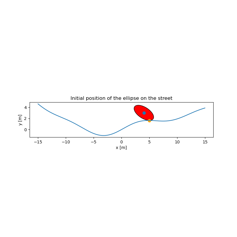
Slope of ellipse and of street should be the same at the contact point:
initial slope of street:  -0.01162
initial slope of ellipse: -0.01162

Ensure that the particle is inside the ellipse.

if alpha1**2/a1**2 + beta1**2/b1**2 >= 1.:
    raise ValueError('Particle is outside the ellipse')

Ensure that the ellipse will touch the street at exactly one point only. find the largest admissible r_max, given strasse, amplitude, frequenz.

r_max = max(a1**2/b1, b1**2/a1)  # max osculating circle of an ellipse


def func2(x, args):
    # just needed to get the arguments matching for minimize
    return np.abs(r_max_lam(x, *args))


x0 = 0.1            # initial guess
minimal = minimize(func2, x0, pL_vals)
if r_max < (x111 := minimal.get('fun')):
    print(f'selected r_max = {r_max} is less than maximally admissible '
          f'radius = {x111:.2f}, hence o.k.\n')
else:
    print(f'selected r_max {r_max} is larger than admissible radius '
          f'{x111:.2f}, hence NOT o.k.\n')
    raise ValueError('the semi radii of the ellipse are too large')


y0 = [q11, x11, gesamt_lam(x11, amplitude1, frequenz1), mx1, my1] + \
     [u11] + initial_speeds
print('initial conditions are:')
for i in range(len(y0)):
    print(f"{str(qL[i])} = {y0[i]:.3f}")


def gradient(t, y, args):
    sol = np.linalg.solve(MM_lam(*y, *args), force_lam(*y, *args))
    return np.array(sol).T[0]


times = np.linspace(0., intervall, schritte)
t_span = (0., intervall)

resultat1 = solve_ivp(gradient, t_span, y0, t_eval=times, args=(pL_vals,),
                      atol=1.e-8, rtol=1.e-8, method='DOP853')
resultat = resultat1.y.T

print(resultat1.message)
print(f'the integration made {resultat1.nfev} function calls.')

selected r_max = 4.0 is less than maximally admissible radius = 4.09, hence o.k.

initial conditions are:
q(t) = 1.000
x(t) = 5.000
y(t) = 1.644
mx(t) = 4.022
my(t) = 3.014
u(t) = 2.500
ux(t) = -4.441
uy(t) = 0.052
umx(t) = -4.539
umy(t) = -2.431
The solver successfully reached the end of the integration interval.
the integration made 9989 function calls.

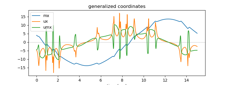
Plot whatever generalized coordinates are of interest.

fig, ax = plt.subplots(figsize=(8, 3))
bezeichnung = ['q', 'x', 'y', 'mx', 'my', 'u', 'ux', 'uy', 'umx', 'umy']
for i in (3, 6, 8):
    ax.plot(times, resultat[:, i], label=bezeichnung[i])
ax.set_xlabel('time (sec)')
ax.axhline(0, color='gray', lw=0.5, linestyle='--')
ax.set_title('generalized coordinates')
_ = ax.legend()

Energy

kin_np = np.empty(schritte)
pot_np = np.empty(schritte)
total_np = np.empty(schritte)

for i in range(schritte):
    kin_np[i] = kin_lam(*[resultat[i, j] for j in range(resultat.shape[1])],
                        *pL_vals)
    pot_np[i] = pot_lam(*[resultat[i, j] for j in range(resultat.shape[1])],
                        *pL_vals)
    total_np[i] = kin_np[i] + pot_np[i]

fig, ax = plt.subplots(figsize=(8, 3))
ax.plot(times, pot_np, label='potential energy')
ax.plot(times, kin_np, label='kinetic energy')
ax.plot(times, total_np, label='total energy')
ax.set_xlabel('time (sec)')
ax.set_ylabel("energy (Nm)")
ax.set_title('Energies of the system')
ax.legend()
total_max = np.max(total_np)
total_min = np.min(total_np)
print('max deviation of total energy from being constant is {:.2e} % of max'
      ' total energy'.format((total_max - total_min)/total_max * 100))

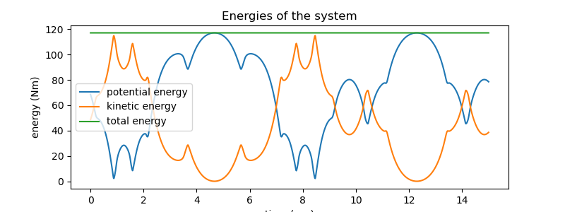
max deviation of total energy from being constant is 1.19e-05 % of max total energy

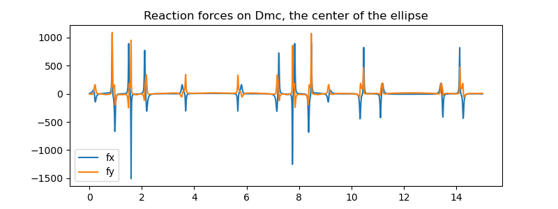
Reaction forces

First \(RHS1 = MM^{-1} \cdot force\) is solved numerically. Then, eingepraegt_lam(…) = 0. for \(f_x, f_y\) is solved. Iteration sometimes helps to improve the results.

RHS1 = np.zeros((schritte, resultat.shape[1]))
for i in range(schritte):
    RHS1[i, :] = np.linalg.solve(
        MM_lam(*[resultat[i, j] for j in range(resultat.shape[1])],
               *pL_vals), force_lam(*[resultat[i, j]
                                      for j in range(resultat.shape[1])],
                                    *pL_vals)).reshape(resultat.shape[1])


def func(x11, *args):
    return eingepraegt_lam(*x11, *args).reshape(len(F))


kraft = np.empty((schritte, len(F)))
x0 = tuple([1. for i in range(len(F))])   # initial guess
for i in range(schritte):
    for _ in range(2):
        y00 = [resultat[i, j] for j in range(resultat.shape[1])]
        RHS2 = [RHS1[i, j] for j in range(RHS1.shape[1])]
        args = tuple((y00 + pL_vals + RHS2))
        A = root(func, x0, args=args)
        x0 = tuple(A.x)  # updated initial guess, may improve convergence
    kraft[i] = A.x

fig, ax = plt.subplots(figsize=(8, 3))
ax.plot(times, kraft[:, 0], label='fx')
ax.plot(times, kraft[:, 1], label='fy')
ax.set_title('Reaction forces on Dmc, the center of the ellipse')
_ = ax.legend()

Animation

fps = 10

t_arr = np.linspace(0.0, intervall, schritte)
state_sol = CubicSpline(t_arr, resultat)

coordinates = Po.pos_from(P0).to_matrix(N)
coords_lam = sm.lambdify(qL + pL, coordinates, cse=True)


def init():
    xmin, xmax = np.min(resultat[:, 1]) - 3., np.max(resultat[:, 1]) + 3.
    ymin, ymax = np.min(resultat[:, 2]) - 3., np.max(resultat[:, 2]) + 3.

    fig = plt.figure(figsize=(10, 10))
    ax = fig.add_subplot(111)
    ax.set_xlim(xmin, xmax)
    ax.set_ylim(ymin, ymax)
    ax.set_aspect('equal')
    ax.grid()

    XX = np.linspace(xmin, xmax,  200)
    ax.plot(XX, gesamt_lam(XX, amplitude1, frequenz1), color='black')

    elli = patches.Ellipse((resultat[0, 3], resultat[0, 4]), width=2.*a1,
                           height=2.*b1, angle=np.rad2deg(resultat[0, 0]),
                           zorder=1, fill=True, color='red', ec='black')
    ax.add_patch(elli)

    line1 = ax.scatter([], [], color='blue', s=30)
    line2 = ax.scatter([], [], color='orange', s=30)
    line3 = ax.scatter([], [], color='black', s=30)
    line4 = ax.axvline(0, color='black', lw=0.75, linestyle='--')
    line5 = ax.axvline(0, color='blue', lw=0.75, linestyle='--')

    return fig, ax, elli, line1, line2, line3, line4, line5


fig, ax, elli, line1, line2, line3, line4, line5 = init()


def update(t):
    message = ((f'Running time {t:.2f} sec \n The black dot is the '
                'particle'))
    ax.set_title(message, fontsize=12)

    elli.set_center((state_sol(t)[3], state_sol(t)[4]))
    elli.set_angle(np.rad2deg(state_sol(t)[0]))
    coords = coords_lam(*[state_sol(t)[j] for j in range(resultat.shape[1])],
                        *pL_vals).flatten()
    line1.set_offsets((state_sol(t)[3], state_sol(t)[4]))
    line2.set_offsets((state_sol(t)[1], state_sol(t)[2]))
    line3.set_offsets((coords[0], coords[1]))
    line4.set_xdata([state_sol(t)[1], state_sol(t)[1]])
    line5.set_xdata([state_sol(t)[3], state_sol(t)[3]])
    return elli, line1, line2, line3, line4, line5


frames = np.linspace(0, intervall, int(fps * (intervall)))
animation = FuncAnimation(fig, update, frames=frames, interval=1000/fps)
plt.show()

Once Loop Reflect