Heat Equation (betts_10_58)

This is example 10.58 from John T. Betts, Practical Methods for Optimal Control Using Nonlinear Programming, 3rd edition, chapter 10: Test Problems. It deals with the ‘discretization’ of a PDE.

Note:

• While it converges rapidly to a solution, the objective value achieved is substantially different from that reported in the book.

States

• \(y_0, .....y_9, w\) : state variables

Specifieds

• \(v, q_{00}, q_{11}\) : control variables

import numpy as np
import sympy as sm
import sympy.physics.mechanics as me
from opty.direct_collocation import Problem

Equations of Motion.

t = me.dynamicsymbols._t

q = list(me.dynamicsymbols(f'q:{10}'))
uq = [q[i].diff(t) for i in range(10)]
w = me.dynamicsymbols('w')
v, q00, q11 = me.dynamicsymbols('v q00 q11')

Parameters fom the example.

qa = 0.2
gamma = 0.04
h = 10.0
delta = 1.0 / 9.0

Equations of motion as per the book.

eom = sm.Matrix([
    -uq[0] + 1/delta**2 * (q[1] - 2*q[0] + q00),
    *[-uq[i] + 1/delta**2 * (q[i+1] - 2*q[i] + q[i-1]) for i in range(1, 9)],
    -uq[-1] + 1/delta**2 * (q11 - 2*q[-1] + q[-2]),
    -w.diff(t) + 1/gamma * (v - w),
    h*(q[0] - w) - 1/(2*delta)*(q[1] - q00),
    1/(2*delta)*(q11 - q[-2]),
])

Optimization

t0, tf = 0.0, 0.2
num_nodes = 501
interval_value = (tf - t0) / (num_nodes - 1)

state_symbols = q + [w]


def obj(free):
    value1 = 1 / (2 * delta) * (qa - free[num_nodes-1])**2
    value2 = 1 / (2 * delta) * (qa - free[10 * num_nodes - 1])**2
    value3 = 1 / delta * np.sum([(qa - free[(i + 1) * num_nodes - 1])**2
                                 for i in range(1, 9)])
    return value1 + value2 + value3


def obj_grad(free):
    grad = np.zeros_like(free)
    grad[num_nodes - 1] = -1 / delta * (qa - free[num_nodes - 1])
    grad[10 * num_nodes - 1] = -1 / delta * (qa - free[10 * num_nodes - 1])
    for i in range(1, 9):
        grad[(i + 1) * num_nodes - 1] = (-2 / delta *
                                         (qa - free[(i + 1) * num_nodes - 1]))
    return grad


# Specify the symbolic instance constraints and the bound, as per the example.
instance_constraints = (
    *[q[i].func(t0) - 0 for i in range(10)],
    w.func(t0) - 0,
)

bounds = {v: (0.0, 1.0)}

Create the optimization problem.

prob = Problem(
    obj,
    obj_grad,
    eom,
    state_symbols,
    num_nodes,
    interval_value,
    instance_constraints=instance_constraints,
    bounds=bounds,
    time_symbol=t,
)

Give some rough estimates for the trajectories.

initial_guess = np.zeros(prob.num_free)

Find the optimal solution.

solution, info = prob.solve(initial_guess)
print(info['status_msg'])
print(f"Objective value achieved: {info['obj_val']:.4e}, ",
      f"as per the book it is {2.45476113*1.e-3:.4e} \n")

b'Algorithm terminated successfully at a locally optimal point, satisfying the convergence tolerances (can be specified by options).'
Objective value achieved: 1.9996e-01,  as per the book it is 2.4548e-03

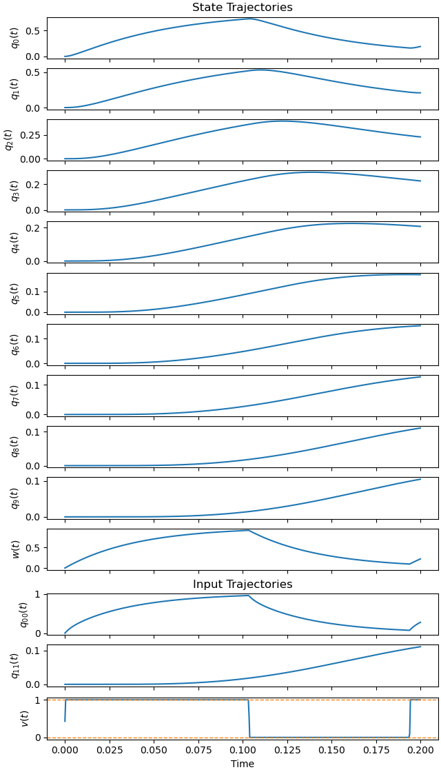
Plot the optimal state and input trajectories.

_ = prob.plot_trajectories(solution, show_bounds=True)

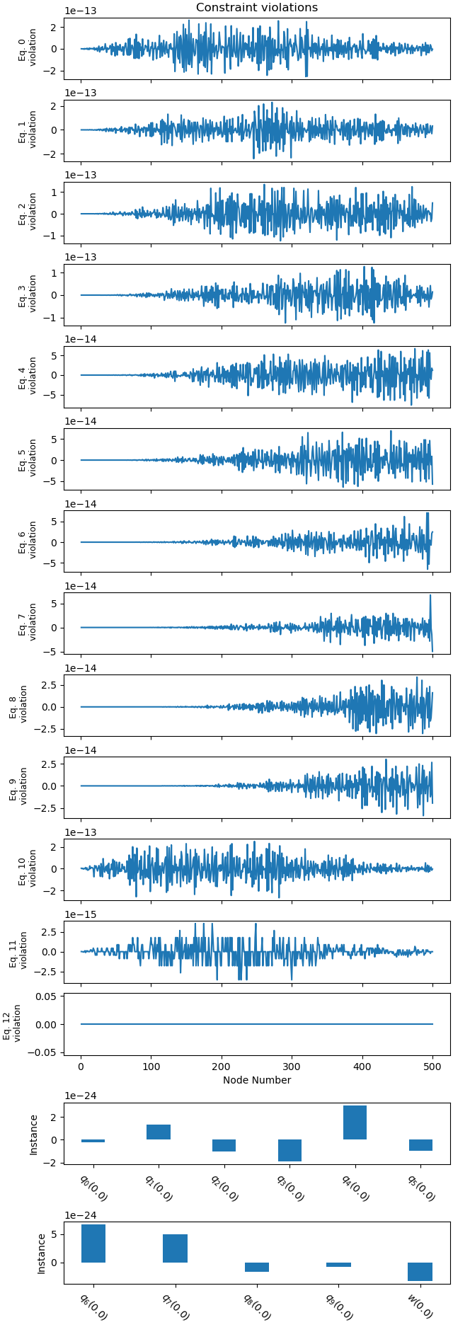
Plot the constraint violations.

_ = prob.plot_constraint_violations(solution, subplots=True)

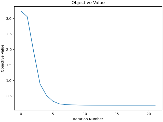
Plot the objective function as a function of optimizer iteration.

_ = prob.plot_objective_value()