Note
Go to the end to download the full example code.
Particle Through Gates
Objective
At present, opty does not allow instance constraints of the form \(x(t_i) - (a, b)\) where \(x\) is a state variable, \(t_i\) is selected by opty and \((a, b)\) is a range for the state variable to be in at the time \(t_i\). This example shows a way to overcome these current limitations.
Introduction
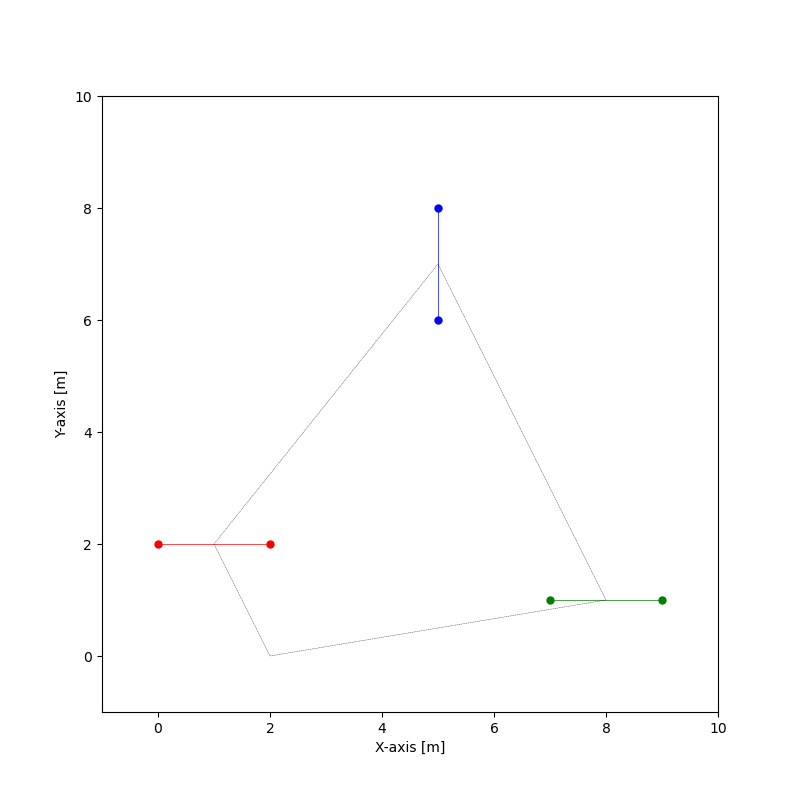
A particle is moving in the horizontal X/Y plane. It is driven by a force \(F = \begin{pmatrix} f_x \\ f_y \end{pmatrix}\) and must pass through three gates. Anywhere inside each gate is allowed, and opty should find the best path and the best times to pass through the gates.
To covercome opty’s current inability one may do as follows:
A: The range limitation:
(For simplicity, the gates are either vertical or horizontal.)
introduce a differentiable hump function \(H(x, a, b, \textrm{steepness})\) that is 1 for \(x \in (a, b)\) else 0. \(\textrm{steepness}\) controls the slopes of the ‘walls’.
introduce state variables \(\textrm{gate}_i\).
add \(\textrm{gate}_i - H(y/x, a_i, b_i, \textrm{steepness}) \cdot \textrm{aux}_i \cdot H(x/y, \textrm{gate}_{i_{x/y}} - \epsilon, \textrm{gate}_{i_{x/y}} + \epsilon, \textrm{steepness})\) to the equations of motion.
\(\textrm{aux}_i \in (0.6, 1.0)\) are free input parameters.
Set \(\textrm{gate}_i = 0.95\) in the instance constraints.
B: The time limitation:
introduce auxiliary state variables \(\textrm{time}_i\), with \(h_i > 0\) and add \(\dfrac{d}{dt}\textrm{time}_i - h_i \cdot \textrm{gate}_i\) to the equations of motion.
This way, \(\textrm{time}_i\) only increases when the particle is near the gate, that is when \(\textrm{gate}_i > 0\). The free parameter \(h_i\) is needed so \(\textrm{time}_i(t_f)\) may be set to 1 in the instance constraints, even if \(0 < \textrm{time}_i < 1\). The larger \(h_i\) the further away the particle may be from the gate, and still \(\textrm{time}_i(t_f) = 1\) will be met. To get convergence, one has to start with a larger value of \(h_i\) and reduce it in the next iterations.
Notes
It is tempting to combine
AandBinto one set of equations of motion, thus reducing the total number of equations of motion from 10 to 7. Both will converge, but the set of 10 equations converges faster. ( 480 sec vs. 70 sec on a standard PC)\(\textrm{steepness} \approx 5.0\) works. If it is too large, convergence seems more difficult.
\(\textrm{aux}_i\) help convergence. Not totally clear, why this is so.
The disadvantage of this approach is that in the example the number of equations of motion raises from 4 to 10.
In the iteration around
Problem / solve, an iteration may end with some error, yet this error is good as intital guess for the next iteration. As I do not know the inner workings of Ipopt I do not know why this works - but it does.If in \(-\textrm{limit} \leq f_x, f_y \leq \textrm{limit}\) the value of \(\textrm{limit}\) is not close to 10.0 it does not converge easily. Unclear why this is so.
States
\(x, y\) are the coordinates of the particle.
\(u_x, u_y\) are the velocities of the particle.
\(\textrm{gate}_i\) auxiliary variables described above.
\(\textrm{time}_i\) auxiliary variables, described above
Known Parameters
\(m\) is the mass of the particle [kg].
\(\nu\) is the friction coefficient [kg/s].
\(a_i, b_i\) are the coordinates of the gates [m].
\(\textrm{steepness}\) as described above.
\(\textrm{gate}_{1y}, \textrm{gate}_{2x}, \textrm{gate}_{3y}\) are the coordinates of the gates [m]. (For simplicity, the gates are either vertical or horizontal, so the gate posts have one common coordinate)
Free Parameters
\(h\) is the time step [s].
\(\textrm{aux}_i\) are the auxiliary parameters described above.
\(h_i\) are the auxiliary parameters described above.
Specifieds
\(f_x, f_y\) are the forces acting on the particle [N].
import numpy as np
import sympy as sm
import sympy.physics.mechanics as me
from opty import Problem
from scipy.interpolate import CubicSpline
import matplotlib.pyplot as plt
from matplotlib.animation import FuncAnimation
Define the differentiable hump function and plot it.
def hump_diff(var, a, b, steepness=5.0):
    """returns a differentiable function that is 1 between a and b"""
    return 0.5 * (sm.tanh(steepness * (var - a)) + sm.tanh(steepness *
                                                           (b - var)))


a, b, var, c = sm.symbols('a b var c')
hump_lam = sm.lambdify((var, a, b, c), hump_diff(var, a, b, c), cse=True)

# ``steepness``  wil be set to ``c`` below.
c = 5.0
XX = np.linspace(-5.0, 5.0, 500)
YY_hump = hump_lam(XX, -1.0, 1.0, c)
fig, ax = plt.subplots(figsize=(6.8, 1.5), layout='constrained')
ax.plot(XX, YY_hump)
ax.set_title(f'Differentiable Heaviside function, steepness ={c}')
ax.axvline(x=-1.0, color='black', linestyle='--', lw=0.5)
ax.axvline(x=1.0, color='black', linestyle='--', lw=0.5)

for i in (0.0, 0.1, 0.3, 0.5, 0.8, 1.0, 1.2, 1.4):
    print(f'value of hump at x = {i} is {hump_lam(i, -1.0, 1.0, c):.5f}')
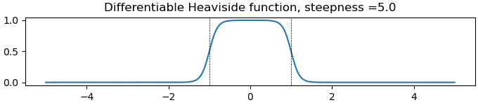
value of hump at x = 0.0 is 0.99991
value of hump at x = 0.1 is 0.99986
value of hump at x = 0.3 is 0.99909
value of hump at x = 0.5 is 0.99331
value of hump at x = 0.8 is 0.88080
value of hump at x = 1.0 is 0.50000
value of hump at x = 1.2 is 0.11920
value of hump at x = 1.4 is 0.01799
Set Up the Equations of Motion
N = me.ReferenceFrame('N')
O, P = sm.symbols('O P', cls=me.Point)

O.set_vel(N, 0)
t = me.dynamicsymbols._t

x, y, ux, uy = me.dynamicsymbols('x y ux uy')
gate_1, gate_2, gate_3 = me.dynamicsymbols('gate_1 gate_2 gate_3')
fx, fy = me.dynamicsymbols('fx, fy')

m, nu = sm.symbols('m nu')
steepness = sm.symbols('steepness')
a1l, a1r, a2b, a2t, a3l, a3r = sm.symbols('a1l a1r a2b a2t a3l a3r')
gate_1y, gate_2x, gate_3y = sm.symbols('gate_1y gate_2x gate_3y')
aux1, aux2, aux3 = sm.symbols('aux1, aux2, aux3')
epsilon = sm.symbols('epsilon')

time1, time2, time3 = me.dynamicsymbols('time1 time2 time3')
h1, h2, h3 = sm.symbols('h1 h2 h3')

P.set_pos(O, x * N.x + y * N.y)
P.set_vel(N, ux * N.x + uy * N.y)

body = me.Particle('body', P, m)
bodies = [body]
forces = [(P, fx * N.x + fy * N.y - nu * P.vel(N))]
kd = sm.Matrix([ux - x.diff(t), uy - y.diff(t)])

kanes = me.KanesMethod(N, q_ind=[x, y], u_ind=[ux, uy], kd_eqs=kd)
fr, frstar = kanes.kanes_equations(bodies, forces)
eom = kd.col_join(fr + frstar)
Add the gate conditions to the equations of motion and print them.
eom_gates = sm.Matrix([
    gate_1 - (hump_diff(x, a1l, a1r, steepness) * aux1
              * hump_diff(y, gate_1y - epsilon, gate_1y + epsilon, steepness)),
    gate_2 - (hump_diff(y, a2b, a2t, steepness) * aux2
              * hump_diff(x, gate_2x - epsilon, gate_2x + epsilon, steepness)),
    gate_3 - (hump_diff(x, a3l, a3r, steepness) * aux3
              * hump_diff(y, gate_3y - epsilon, gate_3y + epsilon, steepness)),
])

eom = eom.col_join(eom_gates)
Add the conditions, so one ‘knows’ that the particle went through the gates.
zeiten = sm.Matrix([time1.diff(t) - h1 * gate_1, time2.diff(t) - h2 * gate_2,
                    time3.diff(t) - h3 * gate_3])

eom = eom.col_join(zeiten)
sm.pprint(eom)
⎡                                                                                      d                               ↪
⎢                                                                              ux(t) - ──(x(t))                        ↪
⎢                                                                                      dt                              ↪
⎢                                                                                                                      ↪
⎢                                                                                      d                               ↪
⎢                                                                              uy(t) - ──(y(t))                        ↪
⎢                                                                                      dt                              ↪
⎢                                                                                                                      ↪
⎢                                                                           d                                          ↪
⎢                                                                       - m⋅──(ux(t)) - ν⋅ux(t) + fx(t)                ↪
⎢                                                                           dt                                         ↪
⎢                                                                                                                      ↪
⎢                                                                           d                                          ↪
⎢                                                                       - m⋅──(uy(t)) - ν⋅uy(t) + fy(t)                ↪
⎢                                                                           dt                                         ↪
⎢                                                                                                                      ↪
⎢-aux₁⋅(0.5⋅tanh(steepness⋅(-a1l + x(t))) + 0.5⋅tanh(steepness⋅(a1r - x(t))))⋅(0.5⋅tanh(steepness⋅(ε - gate_1y + y(t)) ↪
⎢                                                                                                                      ↪
⎢ -aux₂⋅(0.5⋅tanh(steepness⋅(-a2b + y(t))) + 0.5⋅tanh(steepness⋅(a2t - y(t))))⋅(0.5⋅tanh(steepness⋅(ε - gate₂ₓ + x(t)) ↪
⎢                                                                                                                      ↪
⎢-aux₃⋅(0.5⋅tanh(steepness⋅(-a3l + x(t))) + 0.5⋅tanh(steepness⋅(a3r - x(t))))⋅(0.5⋅tanh(steepness⋅(ε - gate_3y + y(t)) ↪
⎢                                                                                                                      ↪
⎢                                                                                        d                             ↪
⎢                                                                         -h₁⋅gate₁(t) + ──(time₁(t))                  ↪
⎢                                                                                        dt                            ↪
⎢                                                                                                                      ↪
⎢                                                                                        d                             ↪
⎢                                                                         -h₂⋅gate₂(t) + ──(time₂(t))                  ↪
⎢                                                                                        dt                            ↪
⎢                                                                                                                      ↪
⎢                                                                                        d                             ↪
⎢                                                                         -h₃⋅gate₃(t) + ──(time₃(t))                  ↪
⎣                                                                                        dt                            ↪

↪                                                         ⎤
↪                                                         ⎥
↪                                                         ⎥
↪                                                         ⎥
↪                                                         ⎥
↪                                                         ⎥
↪                                                         ⎥
↪                                                         ⎥
↪                                                         ⎥
↪                                                         ⎥
↪                                                         ⎥
↪                                                         ⎥
↪                                                         ⎥
↪                                                         ⎥
↪                                                         ⎥
↪                                                         ⎥
↪ ) + 0.5⋅tanh(steepness⋅(ε + gate_1y - y(t)))) + gate₁(t)⎥
↪                                                         ⎥
↪ ) + 0.5⋅tanh(steepness⋅(ε + gate₂ₓ - x(t)))) + gate₂(t) ⎥
↪                                                         ⎥
↪ ) + 0.5⋅tanh(steepness⋅(ε + gate_3y - y(t)))) + gate₃(t)⎥
↪                                                         ⎥
↪                                                         ⎥
↪                                                         ⎥
↪                                                         ⎥
↪                                                         ⎥
↪                                                         ⎥
↪                                                         ⎥
↪                                                         ⎥
↪                                                         ⎥
↪                                                         ⎥
↪                                                         ⎥
↪                                                         ⎦
Define the Problem and Solve It
h = sm.symbols('h')
num_nodes = 501
state_symbols = (x, y, ux, uy, gate_1, gate_2, gate_3, time1, time2, time3)
t0, t1, t2, t3, tf = (0.0, int(num_nodes/4) * h, int(num_nodes/2) * h,
                      int(3*num_nodes/4) * h, (num_nodes-1) * h)
interval_value = h

par_map = {}
par_map[steepness] = c
par_map[m] = 1.0
par_map[nu] = 0.0
par_map[a1l] = 0.0
par_map[a1r] = 2.0
par_map[a2b] = 6.0
par_map[a2t] = 8.0
par_map[a3l] = 7.0
par_map[a3r] = 9.0
par_map[gate_1y] = 2.0
par_map[gate_2x] = 5.0
par_map[gate_3y] = 1.0
par_map[epsilon] = 0.5

instance_constraints = (
    x.func(t0) - 2.0,
    y.func(t0) - 0.0,
    ux.func(t0) - 0.0,
    uy.func(t0) - 0.0,
    time1.func(t0) - 0.0,
    time2.func(t0) - 0.0,
    time3.func(t0) - 0.0,
    # At the final time particle to be at rest at its starting position.
    x.func(tf) - 2.0,
    y.func(tf) - 0.0,
    ux.func(tf) - 0.0,
    uy.func(tf) - 0.0,
    time1.func(tf) - 1.0,
    time2.func(tf) - 1.0,
    time3.func(tf) - 1.0,
)

limit = 10.0
bounds = {
    h: (0.0, 0.5),
    fx: (-limit, limit),
    fy: (-limit, limit),
    x: (0.0, 15.0),
    y: (0.0, 15.0),
    aux1: (0.6, 1.0),
    aux2: (0.6, 1.0),
    aux3: (0.6, 1.0),
    h1: (1.0, 10.0),
    h2: (1.0, 10.0),
    h3: (1.0, 10.0),
    }


def obj(free):
    return free[-1]


def obj_grad(free):
    grad = np.zeros_like(free)
    grad[-1] = 1.0
    return grad


prob = Problem(
    obj,
    obj_grad,
    eom,
    state_symbols,
    num_nodes,
    interval_value,
    known_parameter_map=par_map,
    instance_constraints=instance_constraints,
    time_symbol=t,
    bounds=bounds,
)
Create a good initial guess.
initial_guess = np.ones(prob.num_free) * 0.0
z1 = int(num_nodes/4)

x1 = np.linspace(2.0, (par_map[a3r] + par_map[a3l])/2, z1)
y1 = np.linspace(0.0, par_map[gate_3y], z1)

x2 = np.linspace((par_map[a3r] + par_map[a3l])/2, par_map[gate_2x], z1)
y2 = np.linspace(par_map[gate_3y], (par_map[a2t] + par_map[a2b])/2, z1)

x3 = np.linspace(par_map[gate_2x], (par_map[a1r] + par_map[a1l])/2, z1)
y3 = np.linspace((par_map[a2t] + par_map[a2b])/2, par_map[gate_1y], z1)

x4 = np.linspace((par_map[a1r] + par_map[a1l])/2, 2.0, z1)
y4 = np.linspace(par_map[gate_1y], 0.0, z1)

x_total = np.concatenate((x1, x2, x3, x4))
y_total = np.concatenate((y1, y2, y3, y4))

initial_guess[0: 8*z1] = np.concatenate((x_total, y_total))
Solve the problem
for i in range(5):
# One has to iterate from a simpler problem, larger h_i means
# it may miss the gates a bit, to a harder one.
# As opty presently does not allow to change bounds without setting up
# **Problem** again, one has to do this here.
bounds[h1] = (1.0, 410.0 - i * 100)
bounds[h2] = (1.0, 410.0 - i * 100)
bounds[h3] = (1.0, 410.0 - i * 100)
par_map[epsilon] = 0.1 + 0.1 * i
prob = Problem(
obj,
obj_grad,
eom,
state_symbols,
num_nodes,
interval_value,
known_parameter_map=par_map,
instance_constraints=instance_constraints,
time_symbol=t,
bounds=bounds,
)
prob.add_option('max_iter', 15000)
solution, info = prob.solve(initial_guess)
initial_guess = solution
print(info['status_msg'])
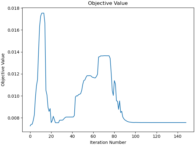
_ = prob.plot_objective_value()
b'Algorithm converged to a point of local infeasibility. Problem may be infeasible.'
b'Algorithm converged to a point of local infeasibility. Problem may be infeasible.'
b'Algorithm terminated successfully at a locally optimal point, satisfying the convergence tolerances (can be specified by options).'
b'Algorithm terminated successfully at a locally optimal point, satisfying the convergence tolerances (can be specified by options).'
b'Algorithm terminated successfully at a locally optimal point, satisfying the convergence tolerances (can be specified by options).'
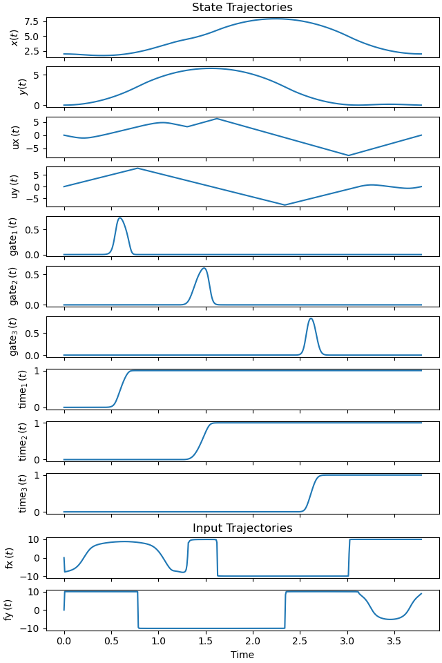
Plot the trajectories.
_ = prob.plot_trajectories(solution)
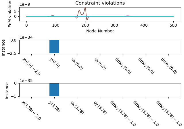
Plot the constraint violations.
_ = prob.plot_constraint_violations(solution)
Print the values of the unknown parameters.
print(f'value of aux1 is {solution[-7]:.5e}')
print(f'value of aux2 is {solution[-6]:.5e}')
print(f'value of aux3 is {solution[-5]:.5e}')
print(f'value of h1 is   {solution[-4]:.5e}')
print(f'value of h2 is   {solution[-3]:.5e}')
print(f'value of h3 is   {solution[-2]:.5e}')
print(f'value of h is    {solution[-1]:.5e}')
value of aux1 is 9.94908e-01
value of aux2 is 9.99989e-01
value of aux3 is 9.99993e-01
value of h1 is   9.94871e+00
value of h2 is   9.99989e+00
value of h3 is   9.99993e+00
value of h is    7.56973e-03
Animate the Simulation
fps = 20

state_vals, input_vals, _, h_sol = prob.parse_free(solution)

tf = h_sol*(num_nodes - 1)
t_arr = np.linspace(t0, tf, num_nodes)
state_sol = CubicSpline(t_arr, state_vals.T)
input_sol = CubicSpline(t_arr, input_vals.T)

coordinates = P.pos_from(O).to_matrix(N)

pl, pl_vals = zip(*par_map.items())
coords_lam = sm.lambdify((*state_symbols, fx, fy, *pl), coordinates, cse=True)

width, height, radius = 0.5, 0.5, 0.5


def init_plot():
    xmin, xmax = -1.0, 10.0
    ymin, ymax = -1.0, 10.0

    fig, ax = plt.subplots(figsize=(8, 8))
    ax.set_xlim(xmin, xmax)
    ax.set_ylim(ymin, ymax)
    ax.set_aspect('equal')
    ax.set_xlabel('X-axis [m]')
    ax.set_ylabel('Y-axis [m]')

    ax.scatter(par_map[a1l], par_map[gate_1y], color='red', s=25)
    ax.scatter(par_map[a1r], par_map[gate_1y], color='red', s=25)
    ax.plot([par_map[a1l], par_map[a1r]], [par_map[gate_1y], par_map[gate_1y]],
            color='red', lw=0.5)

    ax.scatter(par_map[gate_2x], par_map[a2b], color='blue', s=25)
    ax.scatter(par_map[gate_2x], par_map[a2t], color='blue', s=25)
    ax.plot([par_map[gate_2x], par_map[gate_2x]], [par_map[a2b], par_map[a2t]],
            color='blue', lw=0.5)

    ax.scatter(par_map[a3l], par_map[gate_3y], color='green', s=25)
    ax.scatter(par_map[a3r], par_map[gate_3y], color='green', s=25)
    ax.plot([par_map[a3l], par_map[a3r]], [par_map[gate_3y], par_map[gate_3y]],
            color='green', lw=0.5)

    ax.plot(x_total, y_total, color='black', lw=0.25, linestyle='--')

    line, = ax.plot([], [], color='black', lw=0.5)
    point = ax.scatter([], [], color='black', s=100)
    pfeil = ax.quiver([], [], [], [], color='green', scale=55, width=0.002,
                      headwidth=8)
    return fig, ax, point, line, pfeil


fig, ax, point, line, pfeil = init_plot()
koords = []
for zeit in np.arange(t0, tf, 1/fps):
    coords = coords_lam(*state_sol(zeit), *input_sol(zeit), *pl_vals)
    koords.append(coords)


def update(t):
    message = (f'running time {t:0.2f} sec \n The gree arrow shows the force.'
               f'\n The light grey line is the initial guess.')
    ax.set_title(message)
    line.set_data([], [])
    koordinaten = []
    for i, j in enumerate(np.arange(t0, t, 1/fps)):
        if j <= t:
            koordinaten.append(koords[i])
        else:
            break
    line.set_data([koordinaten[i][0, 0] for i in range(len(koordinaten))],
                  [koordinaten[i][1, 0] for i in range(len(koordinaten))])

    coords = coords_lam(*state_sol(t), *input_sol(t), *pl_vals)

    point.set_offsets([coords[0, 0], coords[1, 0]])
    pfeil.set_offsets([coords[0, 0], coords[1, 0]])
    pfeil.set_UVC(input_sol(t)[0], input_sol(t)[1])
    return point, line, pfeil
Create the animation.
fig, ax, point, line, pfeil = init_plot()
anim = FuncAnimation(fig, update,
                     frames=np.arange(t0, tf, 1/fps),
                     interval=1/fps*1000)


plt.show()
WARNING:matplotlib.animation:MovieWriter ffmpeg unavailable; using Pillow instead.
Total running time of the script: (4 minutes 34.814 seconds)